This project explores housing price prediction on the Boston Housing dataset using multiple approaches — from hand-coded gradient descent to deep learning — to understand the fundamentals of regression at every level of abstraction.
Dataset
Source: Boston Housing (Kaggle)
- 506 samples, 13 features, 1 target (
MEDV— median home value in $1000s) - Train/test split: 80/20 (random state 42)
- Preprocessing: z-score standardisation (mean/std computed on the train set only, applied to both)
Features
| Feature | Description |
|---|---|
CRIM | Per capita crime rate by town |
ZN | Proportion of residential land zoned for lots > 25k sqft |
INDUS | Proportion of non-retail business acres per town |
CHAS | Charles River dummy variable (1 if tract bounds river) |
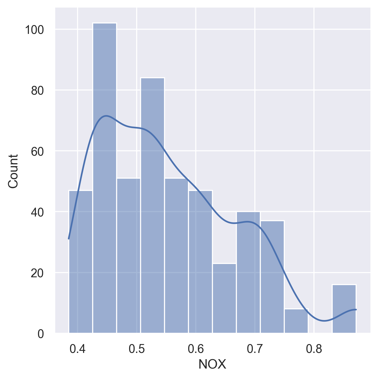
NOX | Nitric oxide concentration (parts per 10 million) |
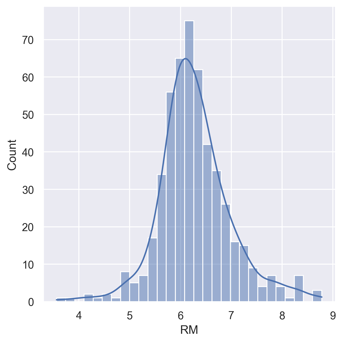
RM | Average number of rooms per dwelling |
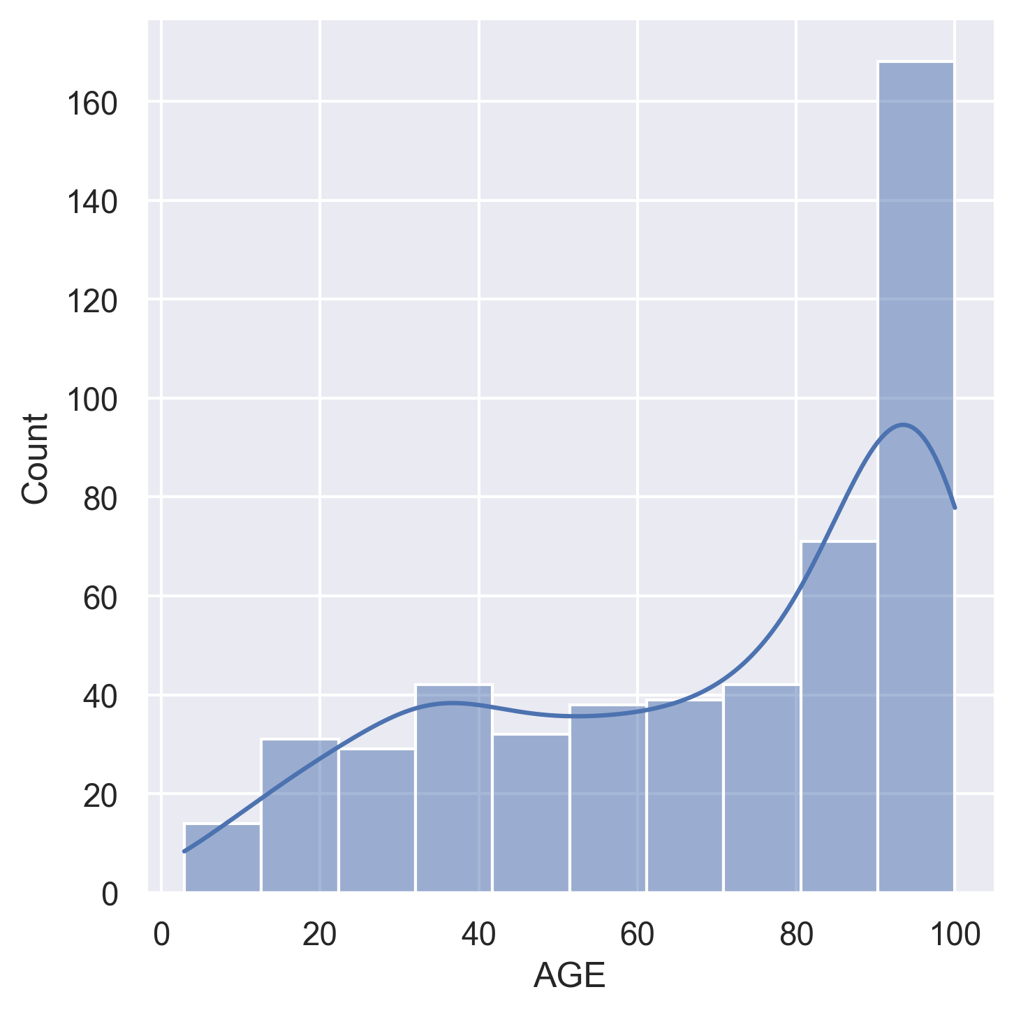
AGE | Proportion of owner-occupied units built pre-1940 |
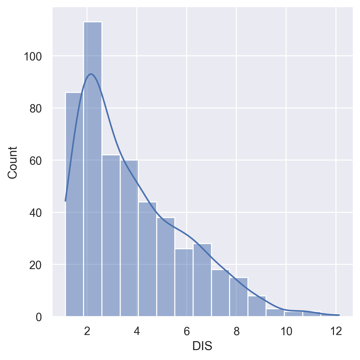
DIS | Weighted distances to five Boston employment centres |
RAD | Index of accessibility to radial highways |
TAX | Full-value property tax rate per $10,000 |
PTRATIO | Pupil-teacher ratio by town |
B | 1000(Bk − 0.63)² where Bk is the proportion of Black residents |
LSTAT | Percentage lower status of the population |
| MEDV | Median value of owner-occupied homes ($1000s) — target |
Dataset Analysis
Feature distributions
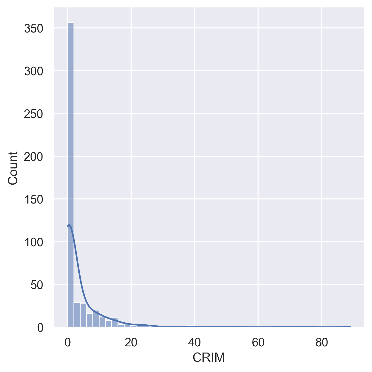
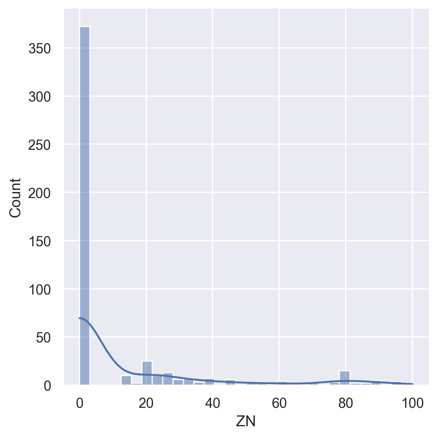
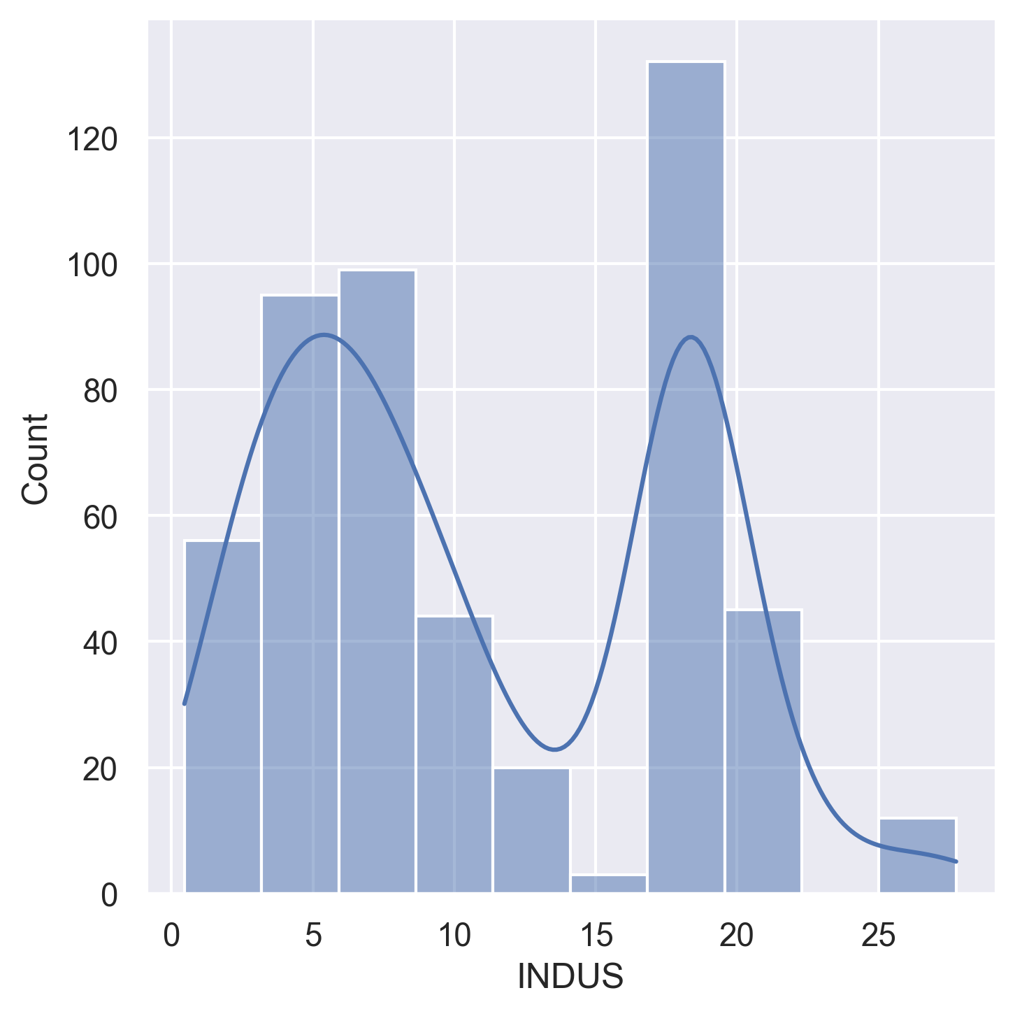
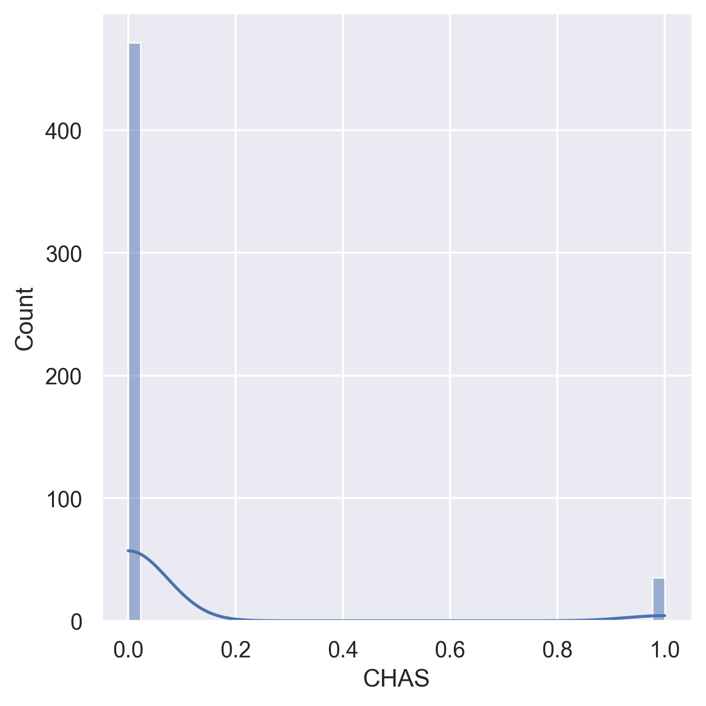
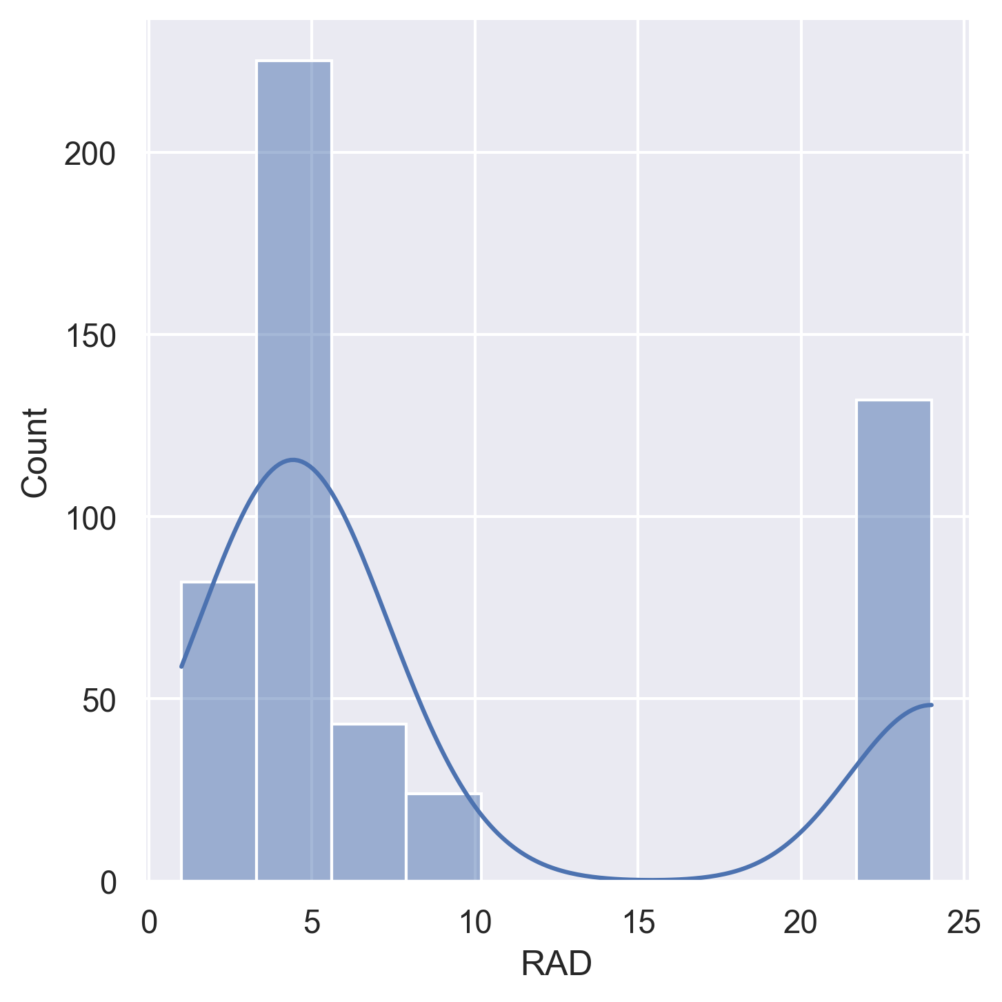
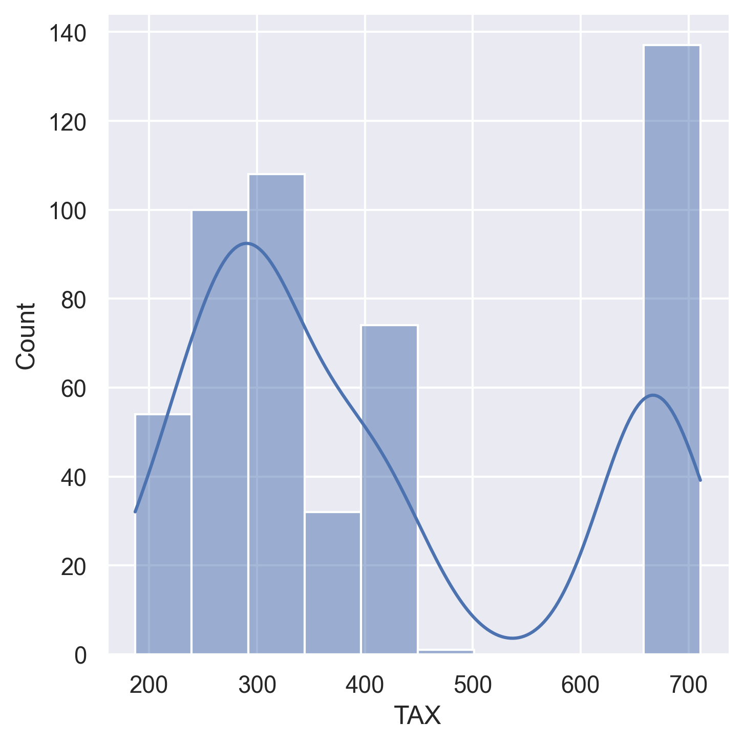
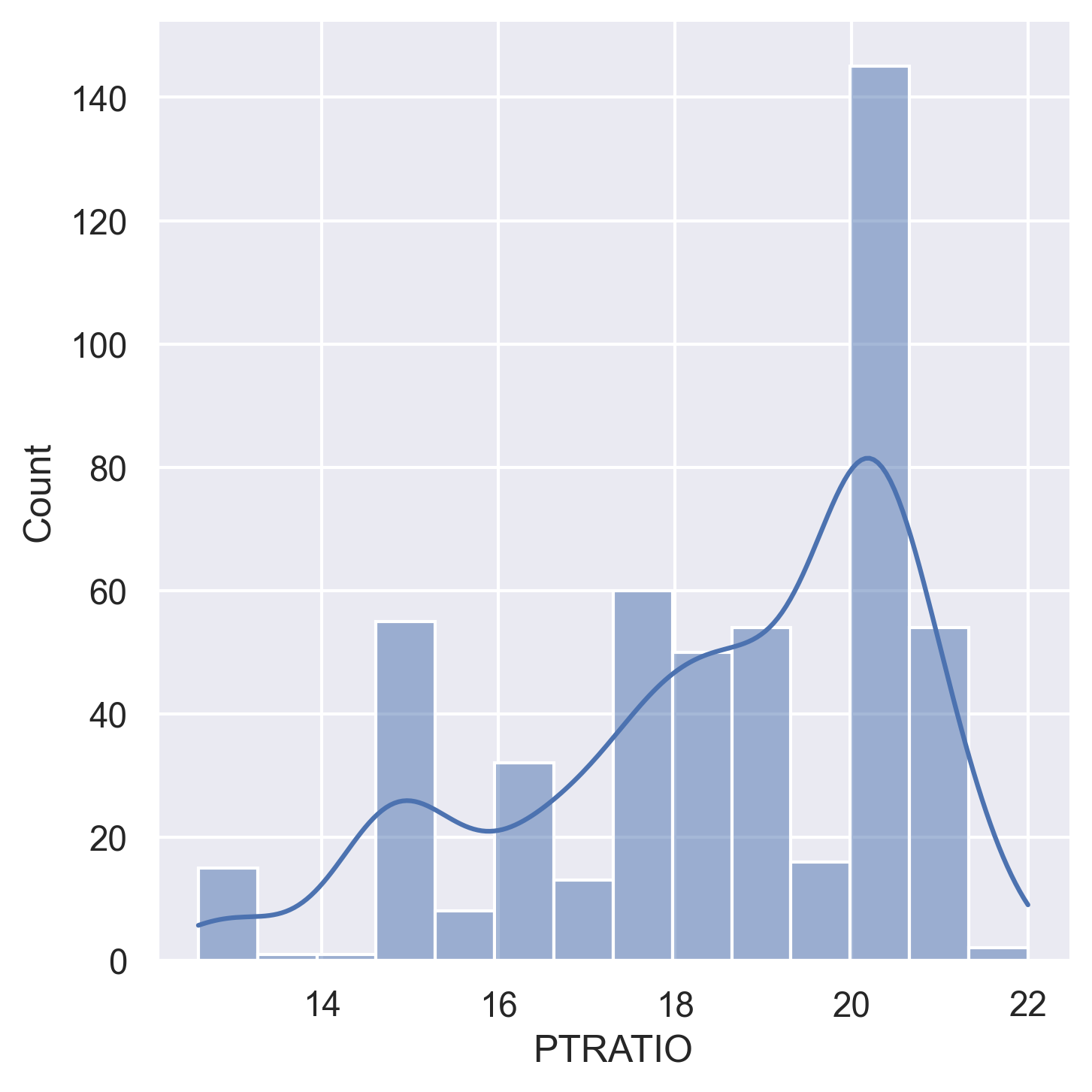
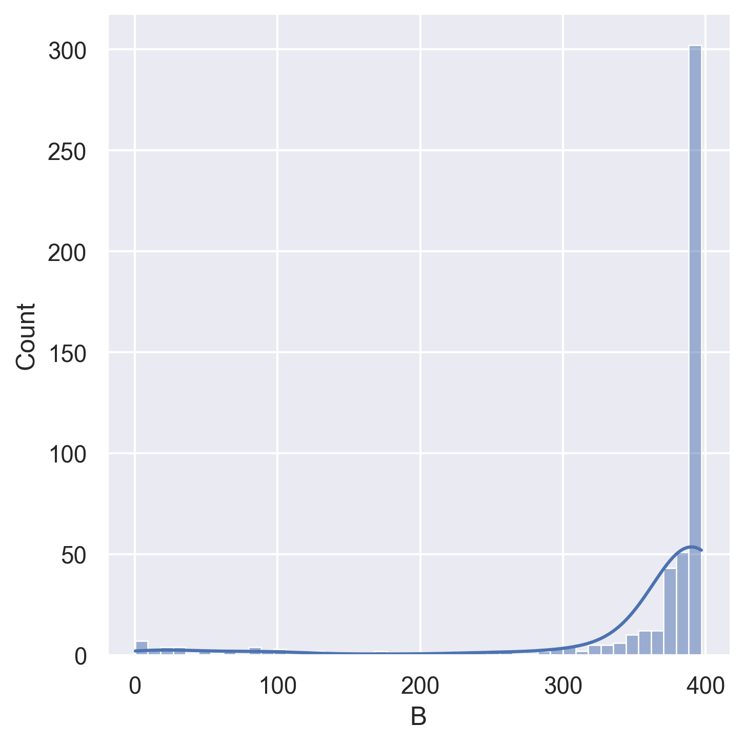
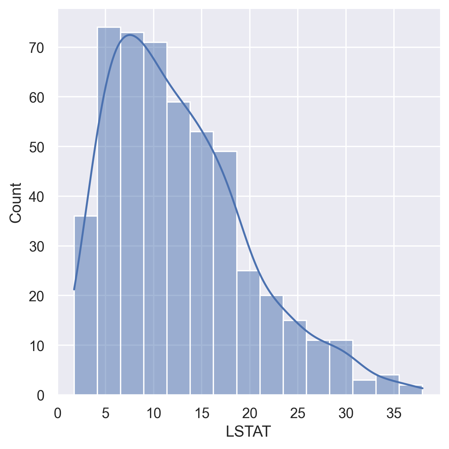
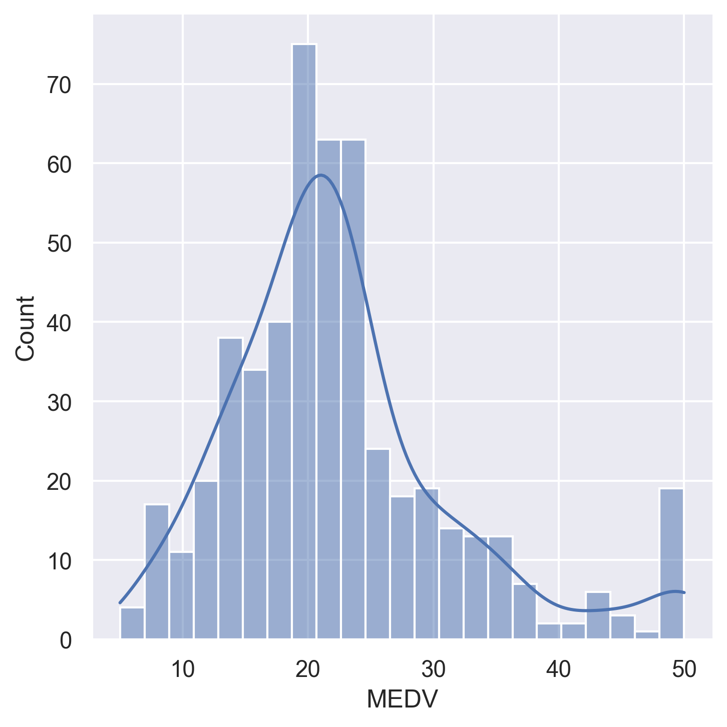
Histograms for all 14 variables in the dataset:
Correlation analysis
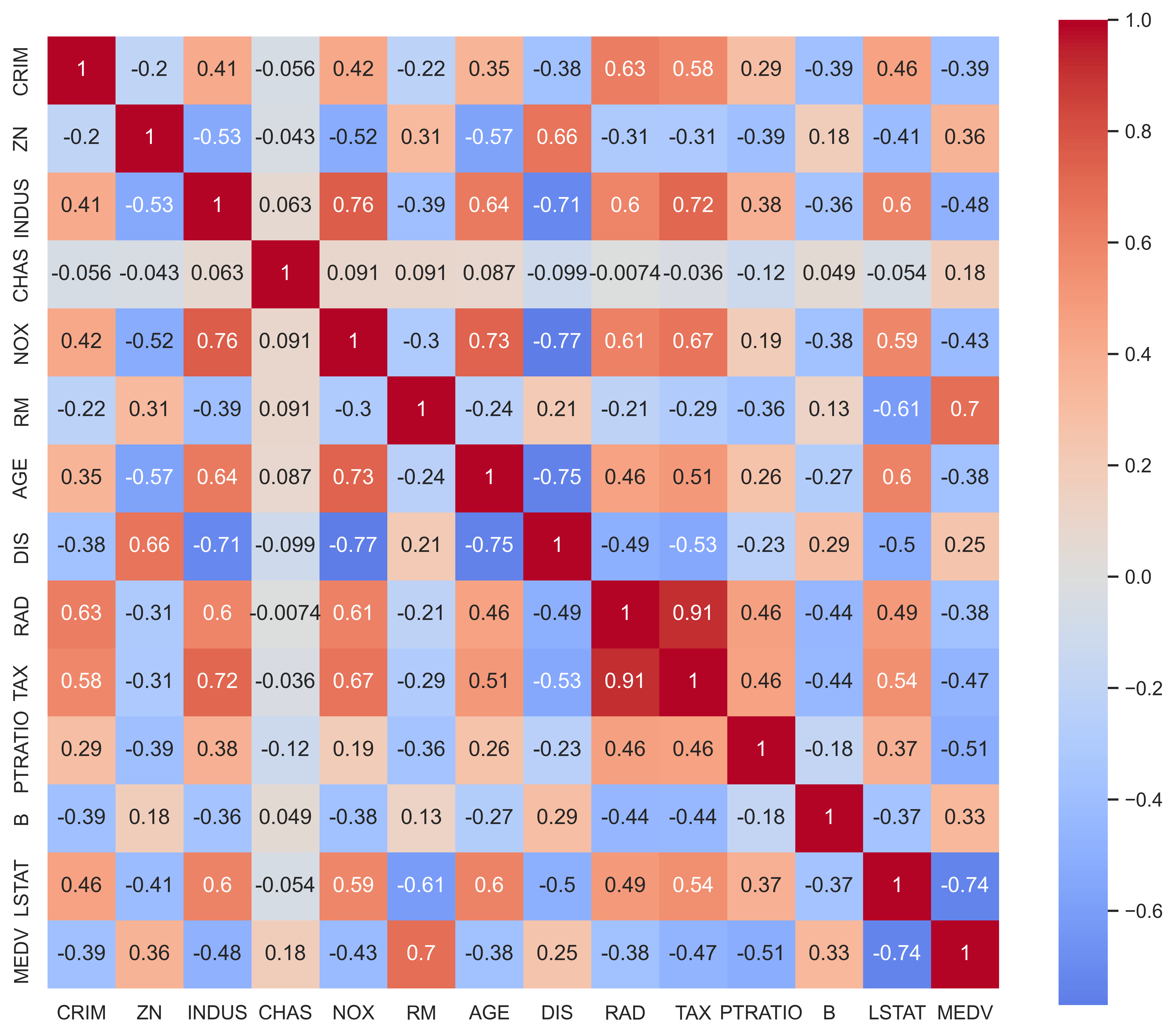
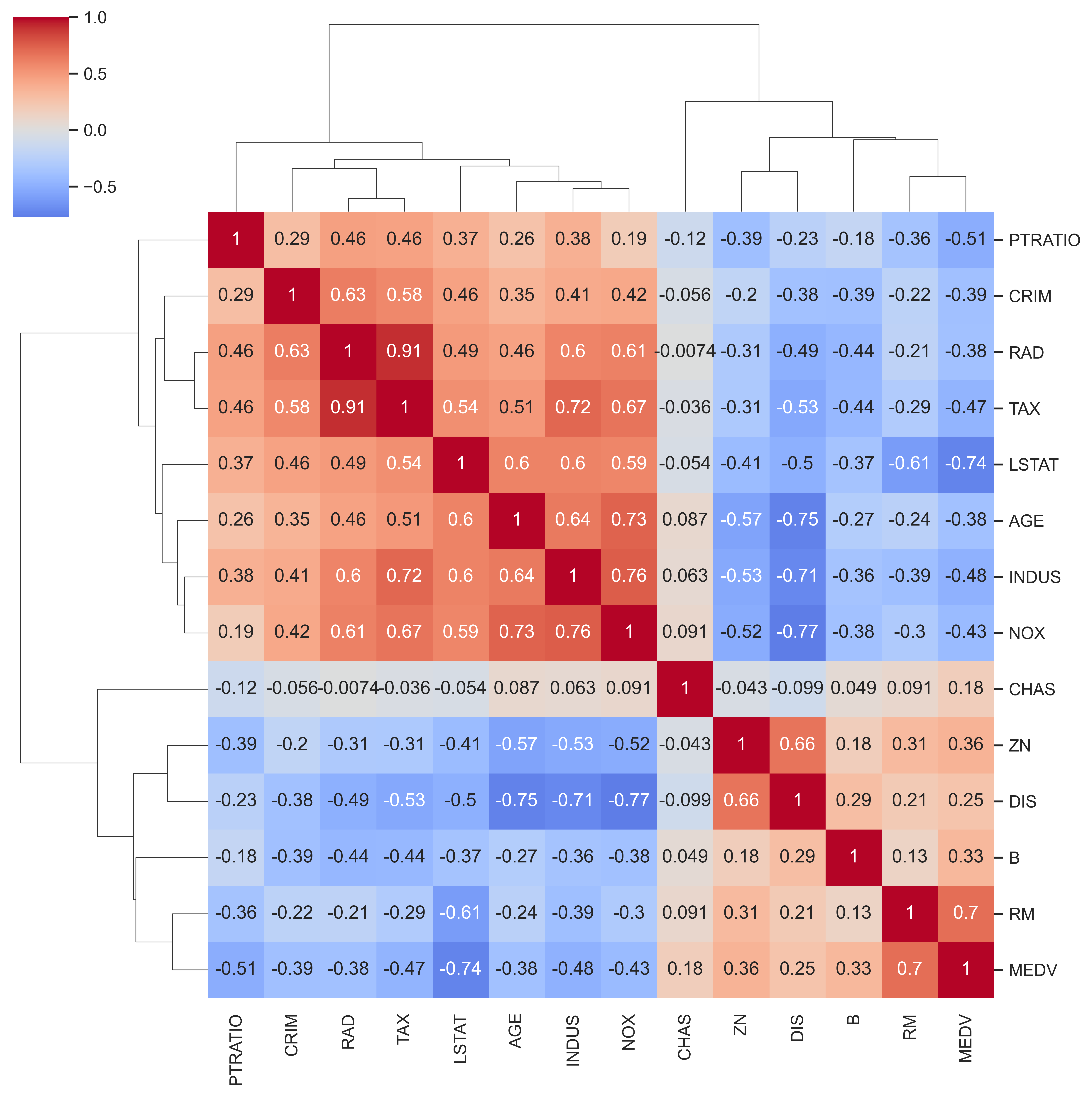
Key correlations with MEDV (target):
- Strong positive:
RM(rooms) — more rooms → higher price - Strong negative:
LSTAT(lower status %) — higher LSTAT → lower price - Notable negatives:
PTRATIO,INDUS,TAX,CRIM
Methods Implemented
1. Gradient descent — linear regression from scratch (rawRun.py)
A pure NumPy implementation with no ML library abstractions:
- Manual weight initialisation (
w ~ N(0, 0.01),b = 0) - MSE loss with analytical gradient computation
- Convergence tolerance check (
tol = 1e-4) - Hyperparameters:
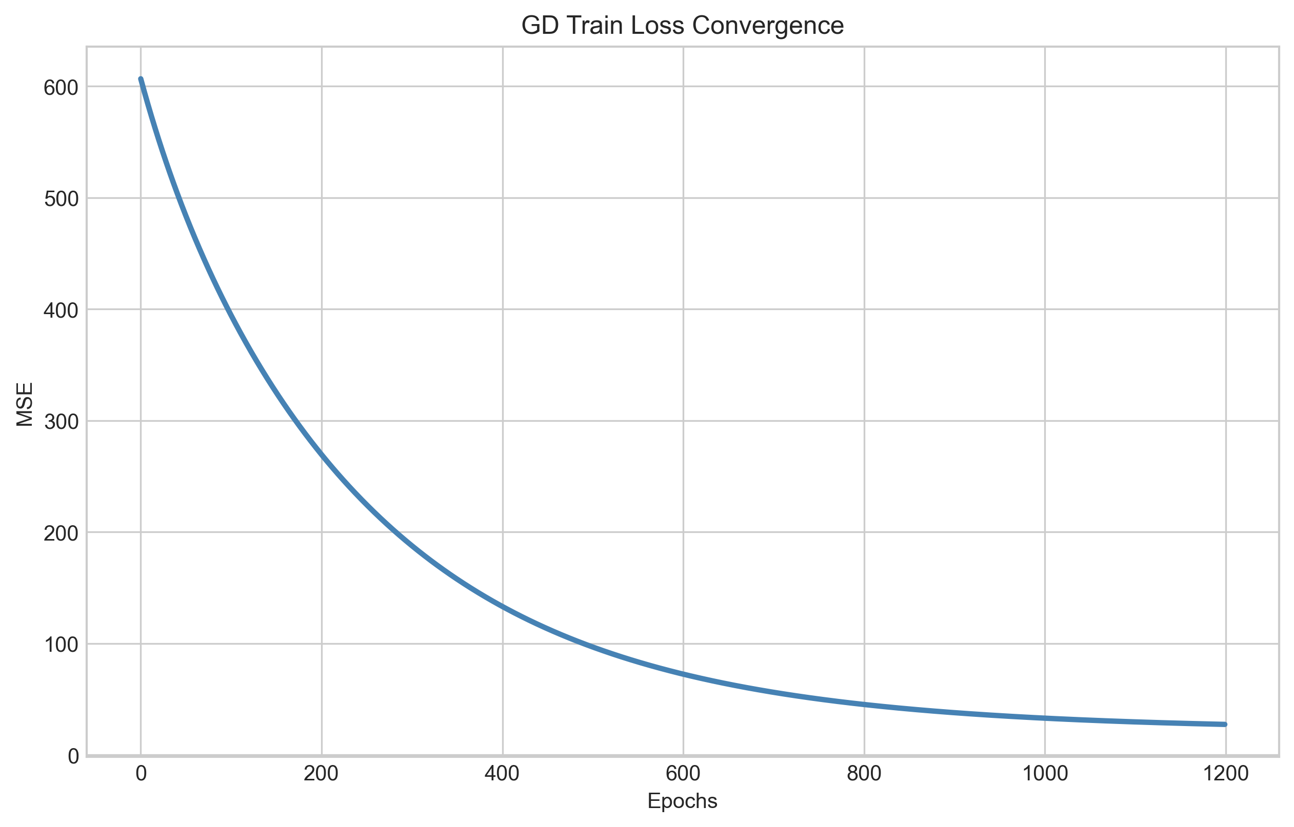
α = 0.001,epochs = 1200
# Core update rule (no libraries)
dw = (2 / m) * X_train.T @ (y_pred - y_train)
db = (2 / m) * sum(y_pred - y_train)
w -= α * dw
b -= α * db
2. Neural network — Keras/TensorFlow (NeuralNetwork.py)
A 3-hidden-layer dense network trained with the Adam optimiser:
| Layer | Units | Activation |
|---|---|---|
| Input | 13 | — |
| Hidden 1 | 22 | ReLU |
| Hidden 2 | 22 | ReLU |
| Hidden 3 | 22 | ReLU |
| Output | 1 | Linear |
- Total parameters: 1,343
- Optimiser: Adam
- Loss: MSE
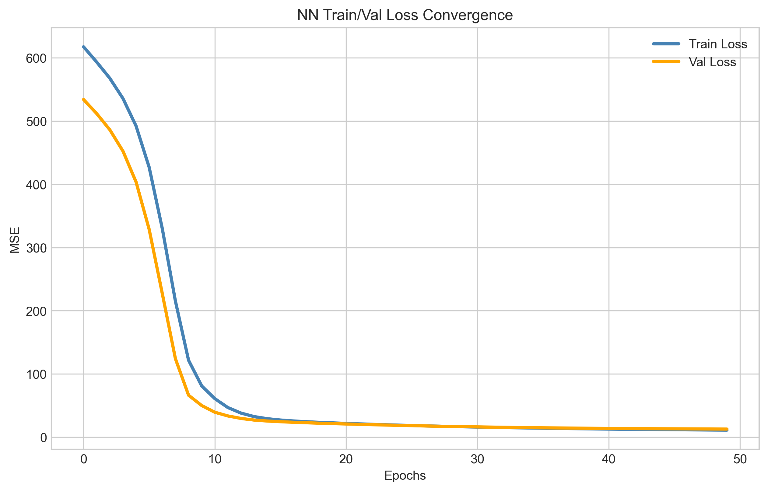
- Batch size: 32, epochs: 50 (with early stopping, patience 20)
3. Evolutionary algorithm (work in progress)
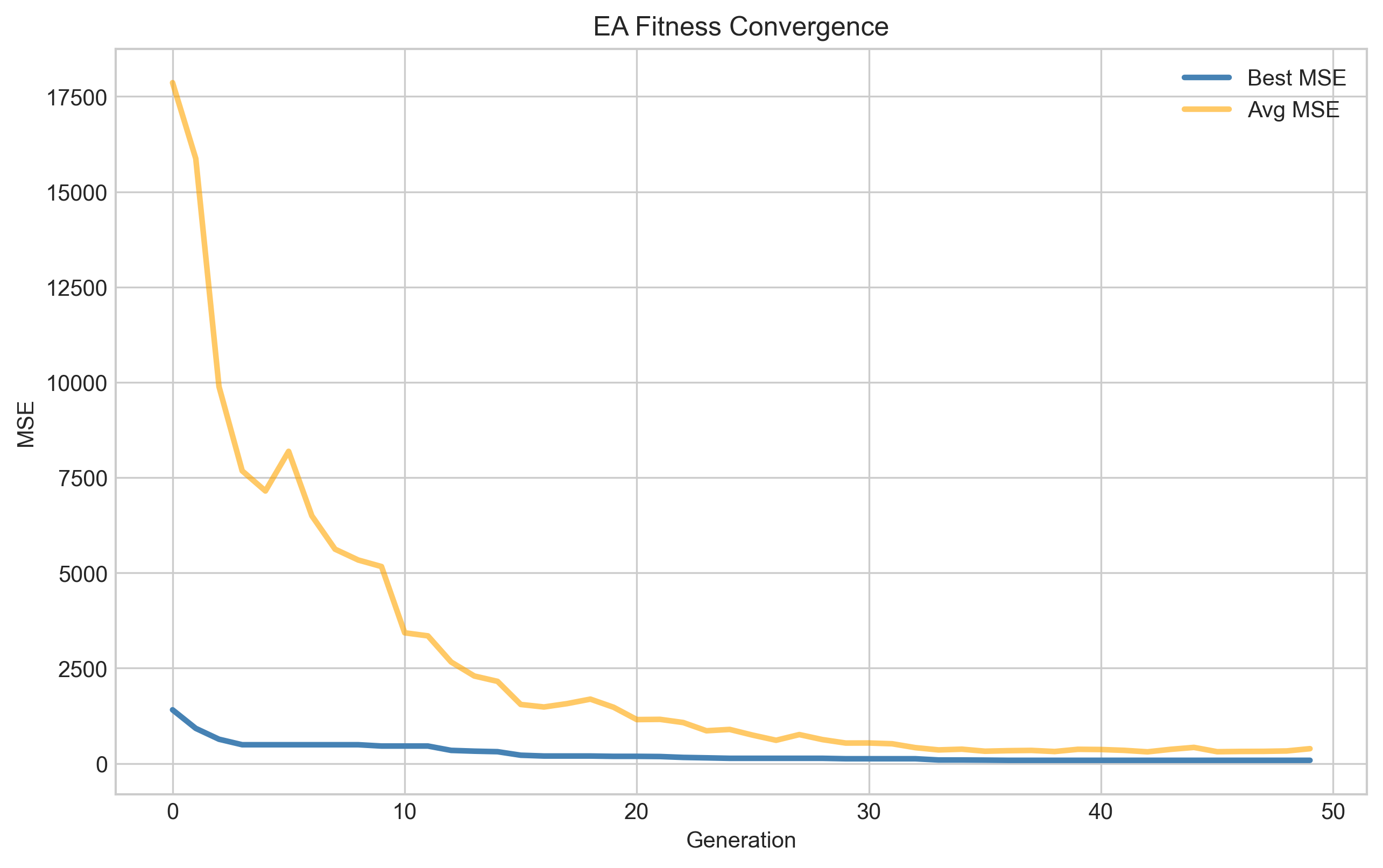
Scaffolded in EvolutionaryAlgorithm.py — evolves neural network weights using:
- Tournament selection (k=3)
- Gaussian mutation (per-gene with configurable rate and sigma)
- Uniform crossover (per-gene swap with configurable rate)
⚠️ Status: skeleton implemented —
fitness(),ea_training_loop()andmutation()are stubbed and awaiting completion.
Results Comparison
Metrics
| Metric | Gradient descent (linear) | Neural network (Keras) | Evolutionary algorithm |
|---|---|---|---|
| MSE | 32.406 | 12.957 | 101.712 |
| RMSE | 5.692 | 3.599 | 10.085 |
| MAE | 3.378 | 2.399 | 7.748 |
| R² | 0.558 | 0.823 | −0.387 |
Training loss curves
Test set predictions — actual vs predicted
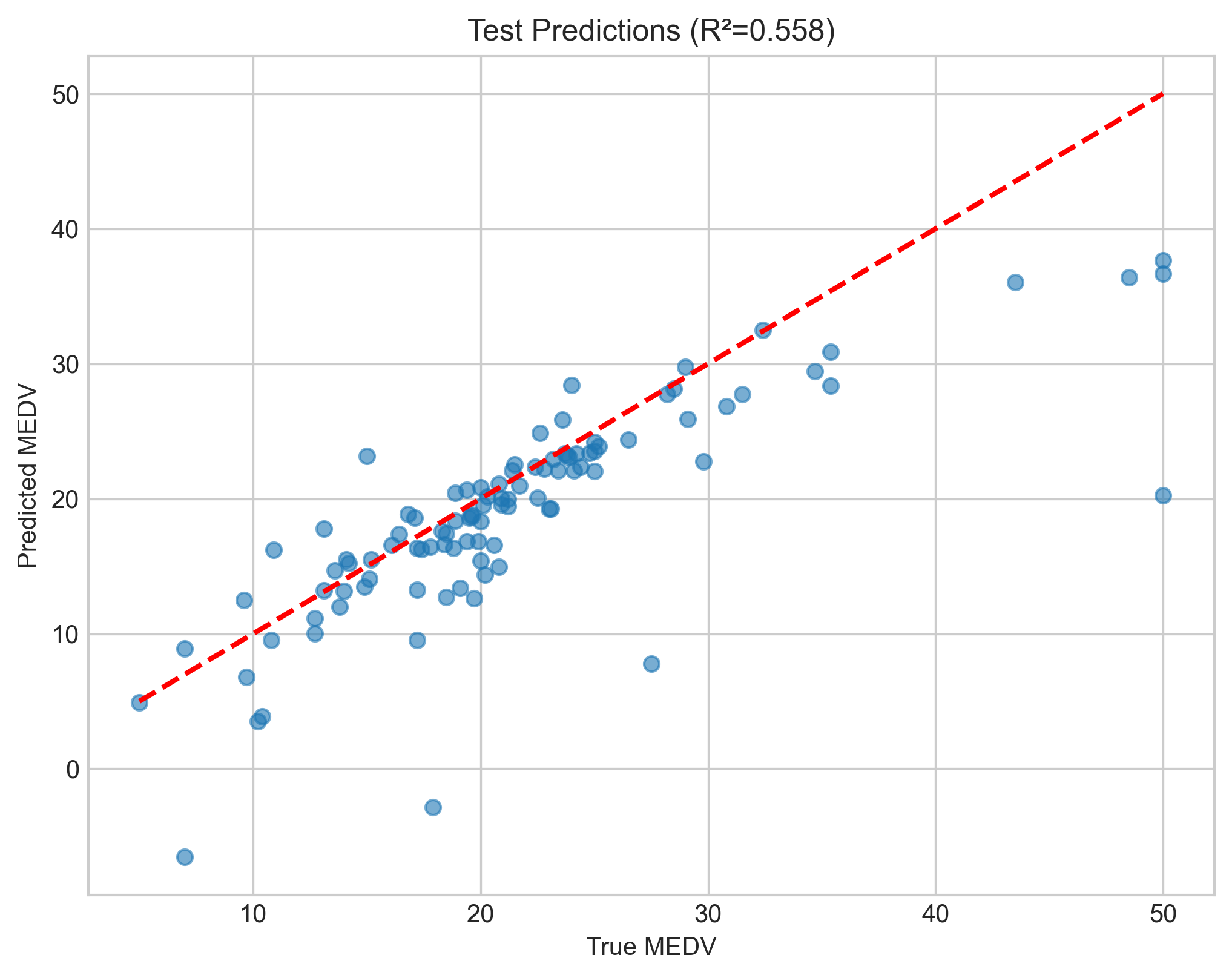
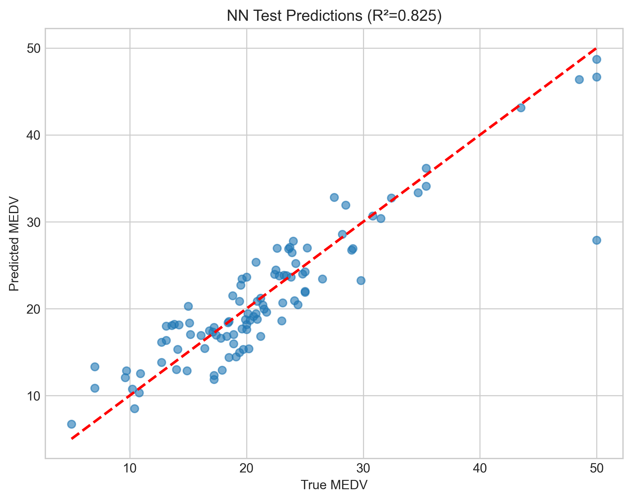
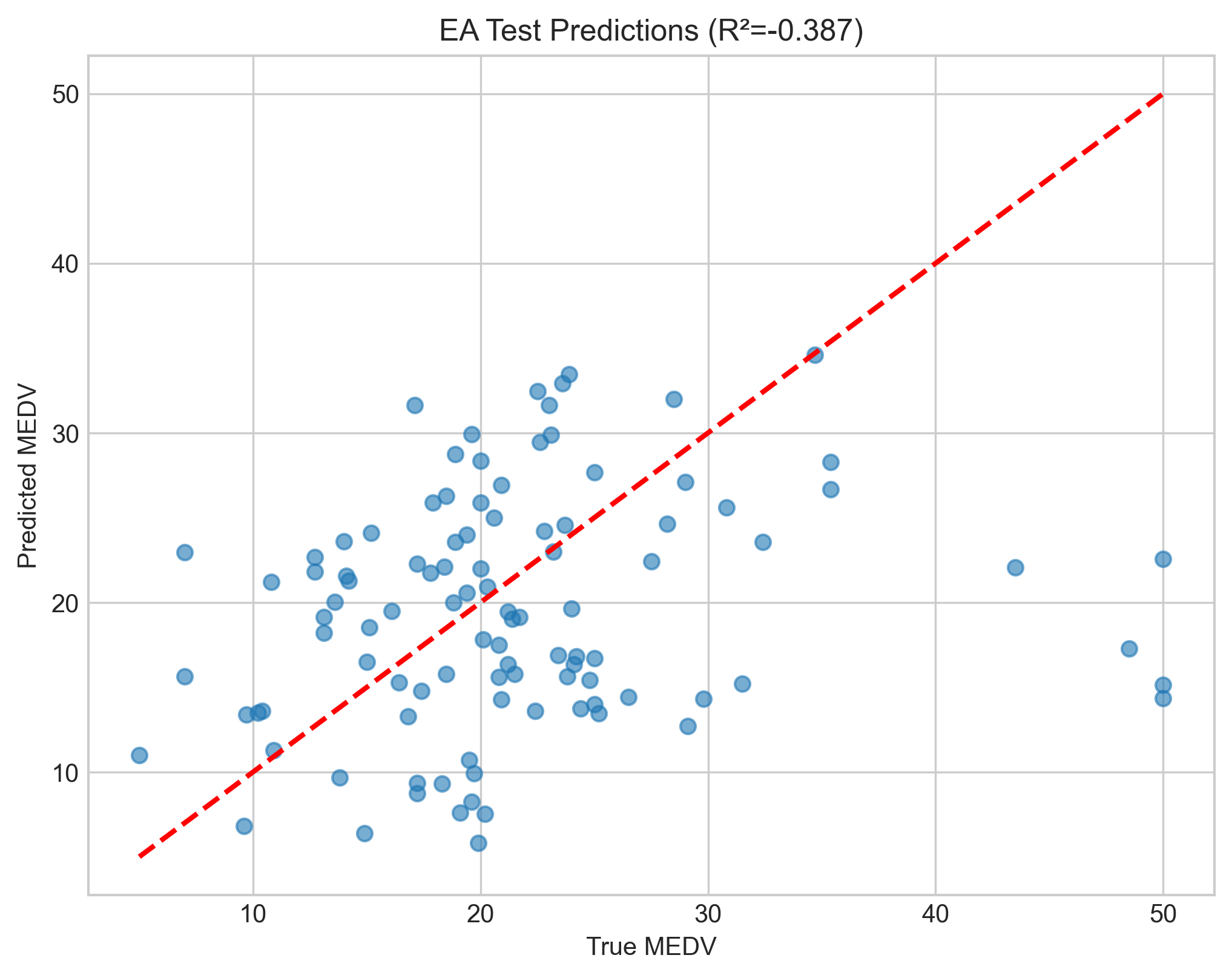
Points closer to the red dashed line (y = x) indicate better predictions. The neural network shows tighter clustering around the ideal line, especially in the mid-range values.
Project Structure
Zamin/
├── rawRun.py                 # Gradient descent linear regression (from scratch)
├── NeuralNetwork.py          # Neural network with Keras/TensorFlow
├── EvolutionaryAlgorithm.py  # Evolutionary algorithm for NN weight optimisation
├── dataPreProcess.py         # Dataset visualisation & correlation analysis
├── housing.csv               # Boston Housing dataset (506 × 14)
├── stickyNote.txt            # Project notes & core concepts
└── output/
    ├── dataanalysis/         # Histograms, heatmaps, correlation plots
    ├── linearreg/            # GD loss curves & scatter plots
    ├── nn/                   # NN loss curves, scatter plots & saved models
    └── ea/                   # EA convergence & prediction plots
Key Takeaways
The evolutionary algorithm failed spectacularly, I was rather surprised. I was expecting it to fall a bit short, but not underperform to this extent. Linear regression and the NN were a delight however — solid scores with very simple setups. I found the NN topology taken from the study to be straightforward to implement and logical.
Future Work
Lots of things could be improved: first and foremost add ridge regression to the linear algorithm, and for the NN add pruning. These are nice, but most of all I will be looking to implement these on a more sophisticated and real-world dataset. This project was great for the rapid feedback loop and small scale. Ramping up to something more fully fledged is the next step. Definitely more to come.