“Back to basics” — Implementing various ML algorithms from scratch with a pure, low-level approach, and coparing them against each other.
Overview
This project explores housing price prediction on the Boston Housing dataset using multiple approaches — from hand-coded gradient descent to deep learning — to understand the fundamentals of regression at every level of abstraction.
Dataset
Source: Boston Housing (Kaggle)
- 506 samples, 13 features, 1 target (
MEDV— Median home value in $1000s) - Train/Test Split: 80/20 (random state 42)
- Preprocessing: Z-score standardisation (mean/std computed on train set only, applied to both)
Features
| Feature | Description |
|---|---|
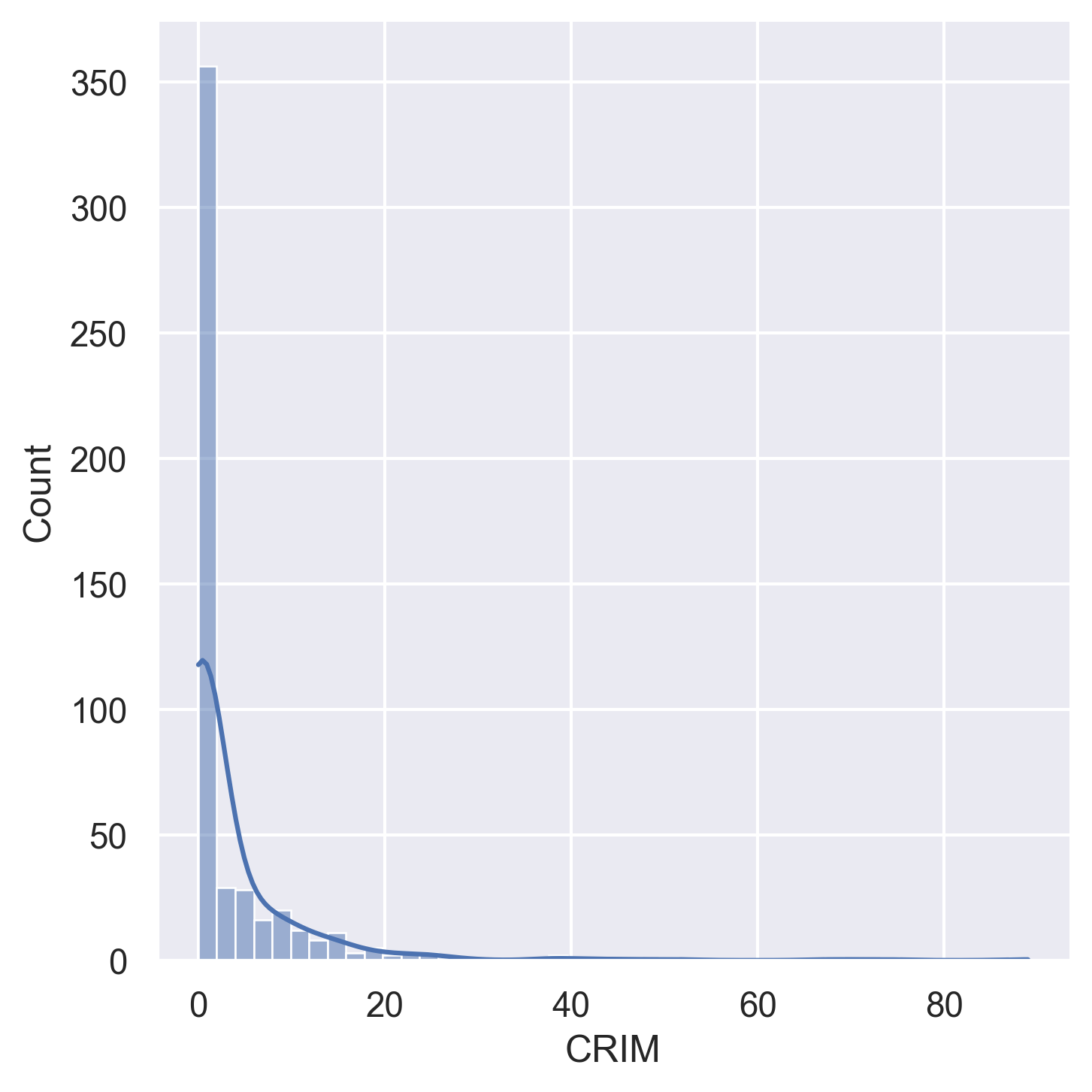
CRIM | Per capita crime rate by town |
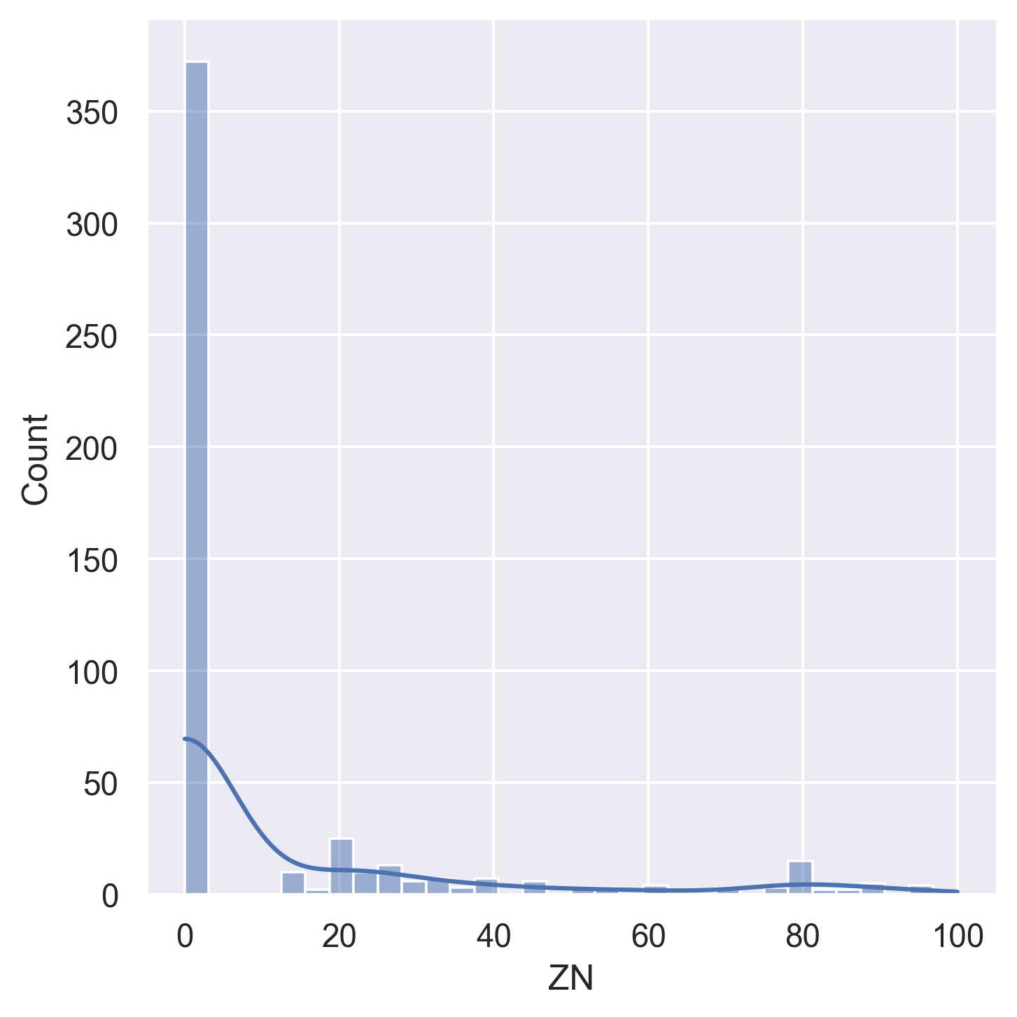
ZN | Proportion of residential land zoned for lots > 25k sqft |
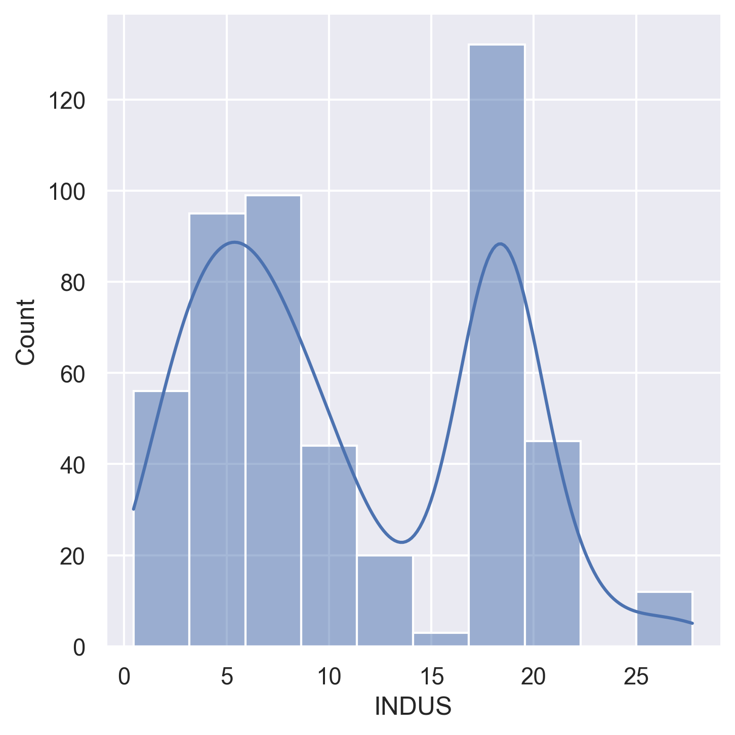
INDUS | Proportion of non-retail business acres per town |
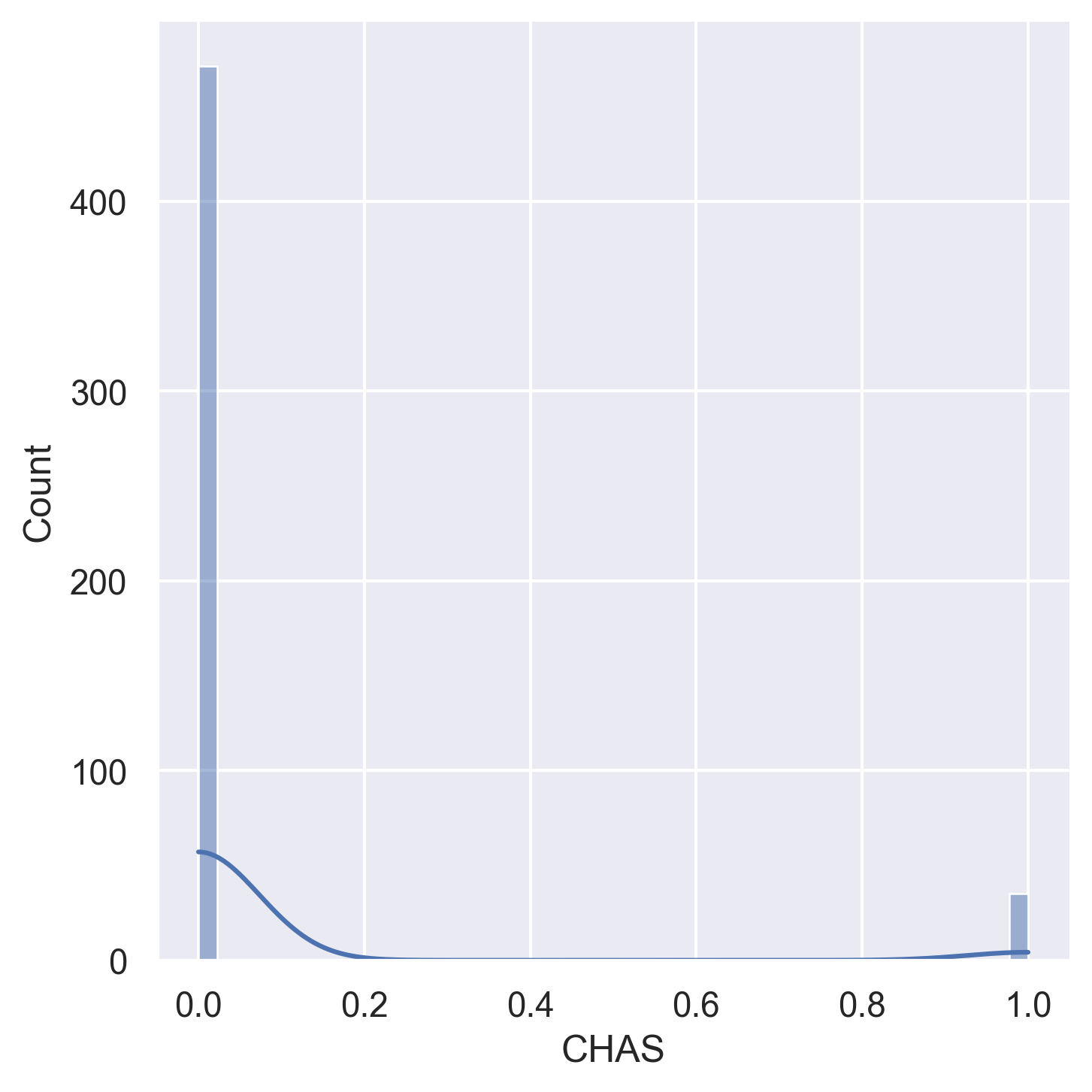
CHAS | Charles River dummy variable (1 if tract bounds river) |
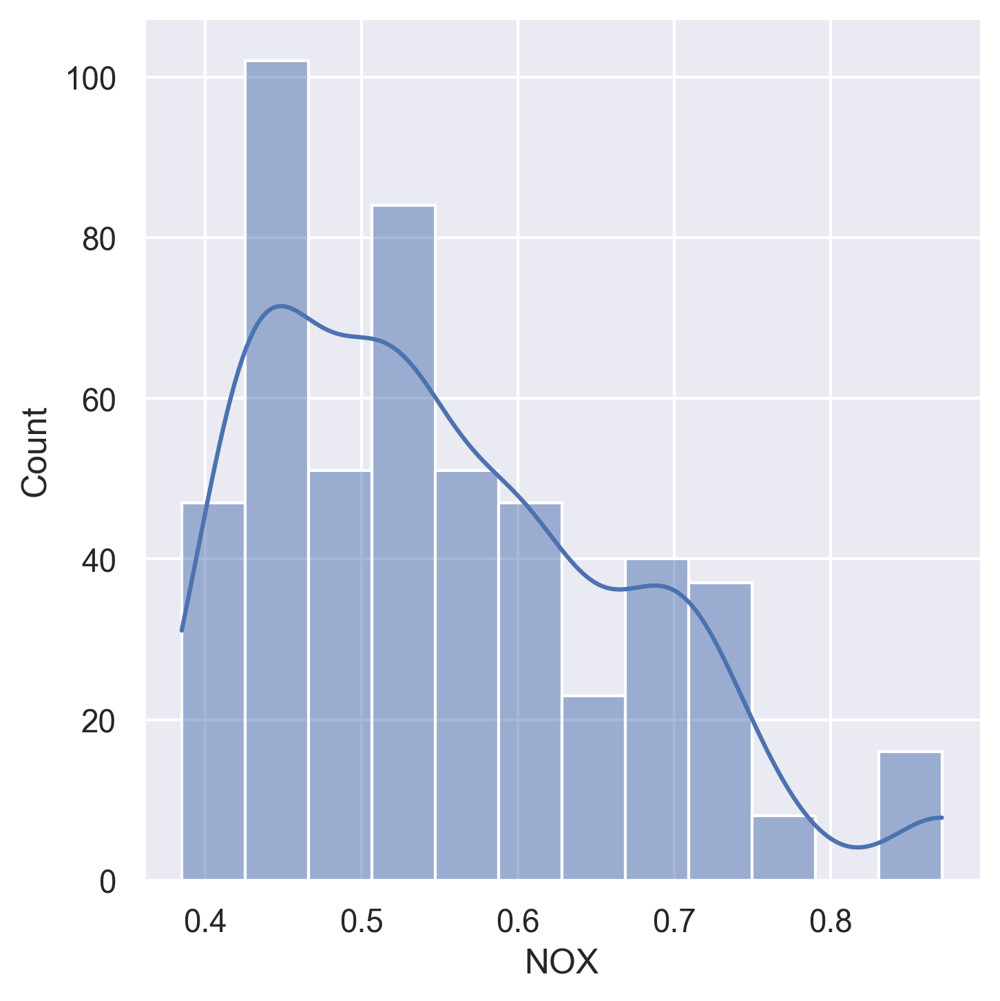
NOX | Nitric oxide concentration (parts per 10 million) |
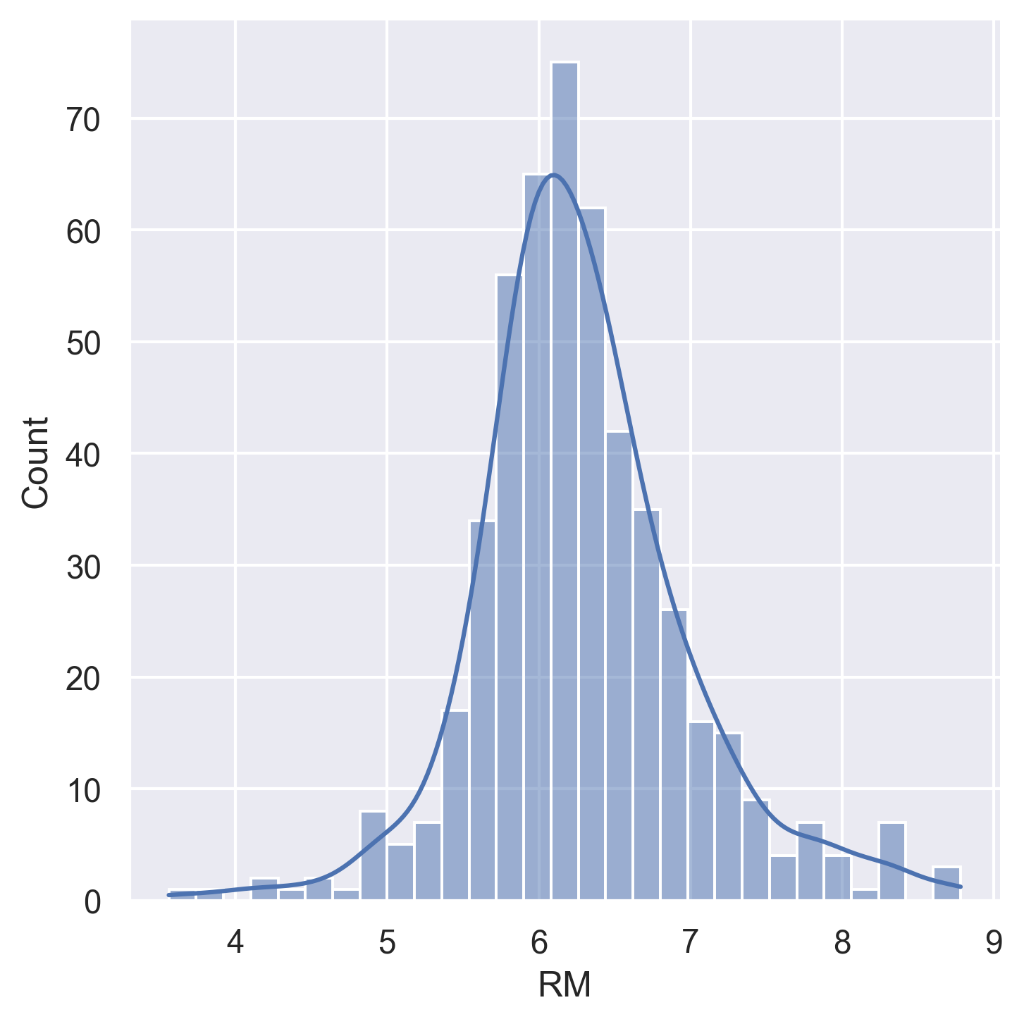
RM | Average number of rooms per dwelling |
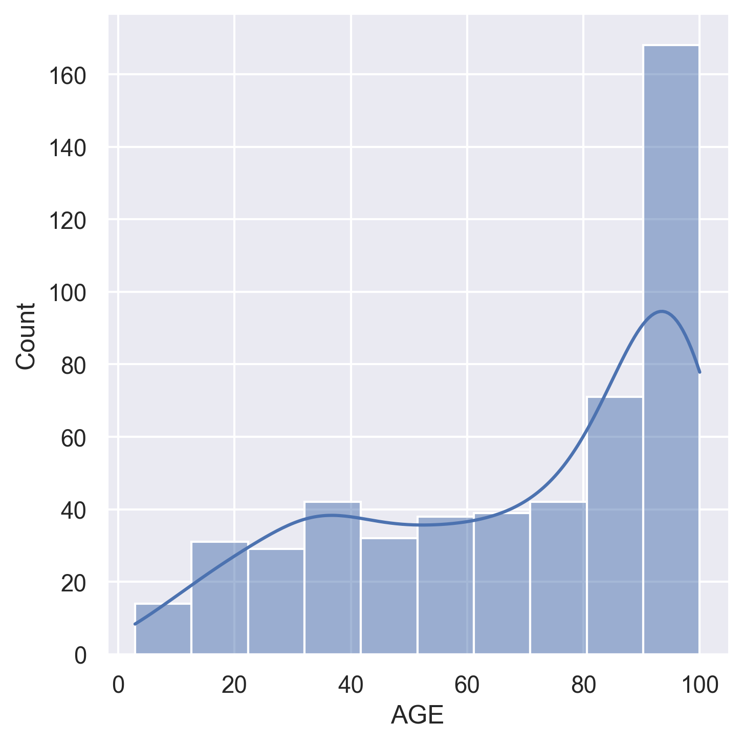
AGE | Proportion of owner-occupied units built pre-1940 |
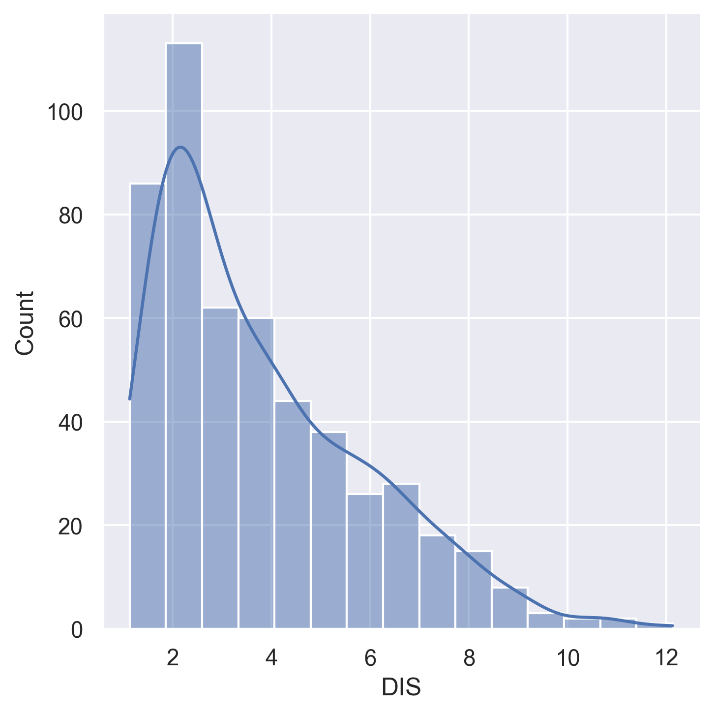
DIS | Weighted distances to five Boston employment centres |
RAD | Index of accessibility to radial highways |
TAX | Full-value property tax rate per $10,000 |
PTRATIO | Pupil-teacher ratio by town |
B | 1000(Bk − 0.63)² where Bk is the proportion of Black residents |
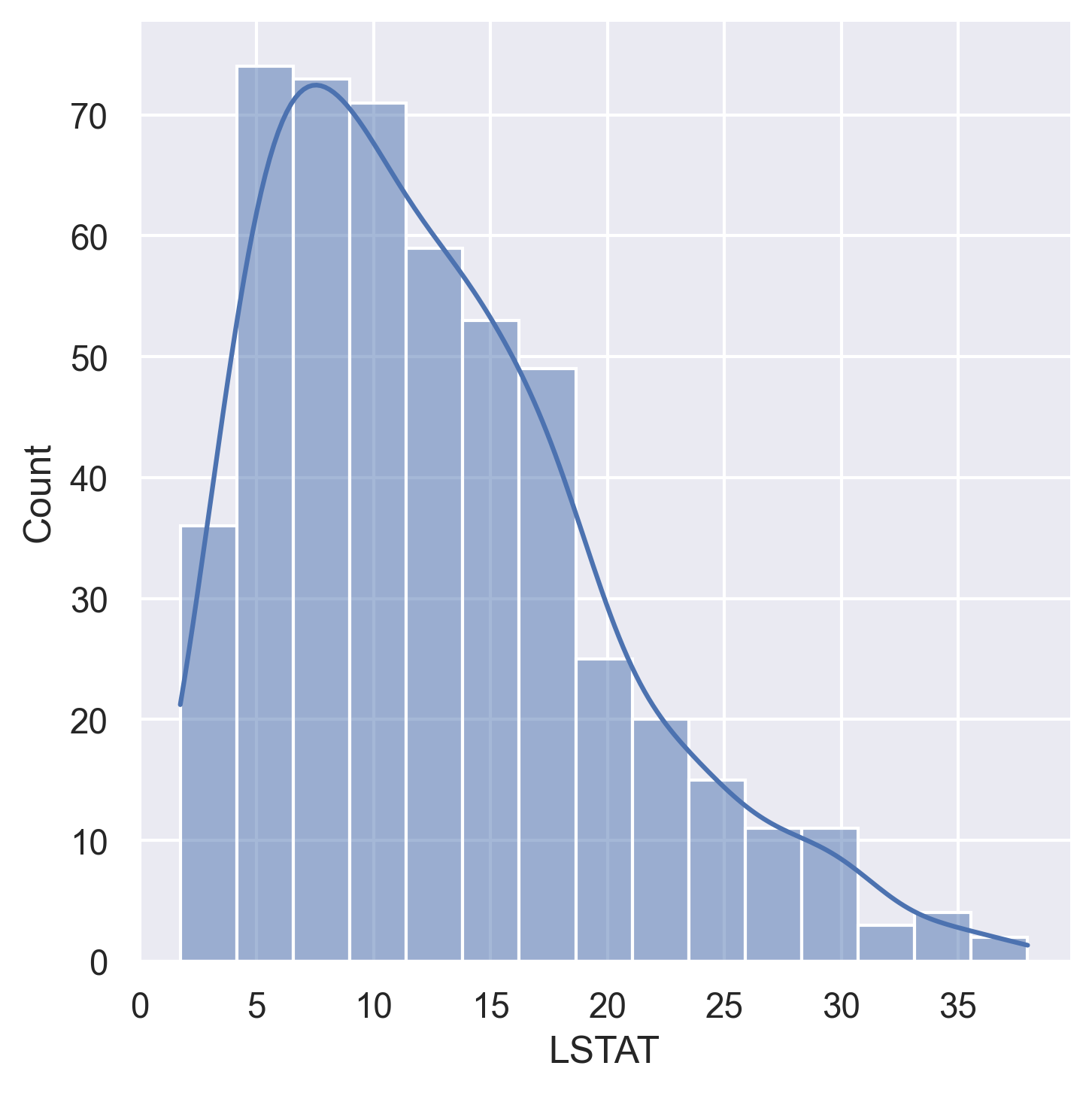
LSTAT | Percentage lower status of the population |
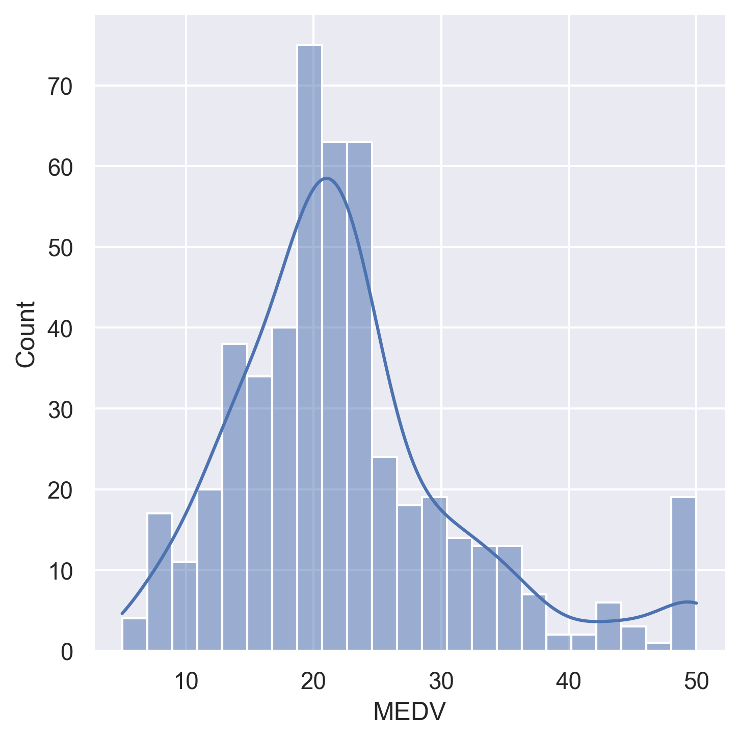
| MEDV | Median value of owner-occupied homes ($1000s) — TARGET |
Dataset Analysis
Feature Distributions
Histograms for all 14 variables in the dataset:
 |  |  |  |
 |  |  |  |
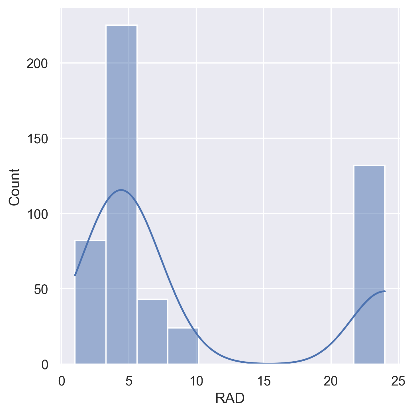 | 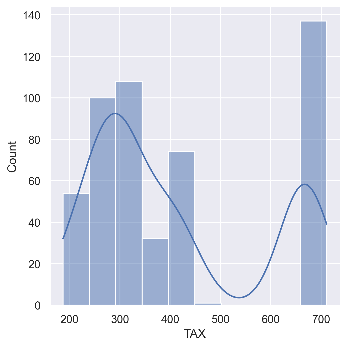 | 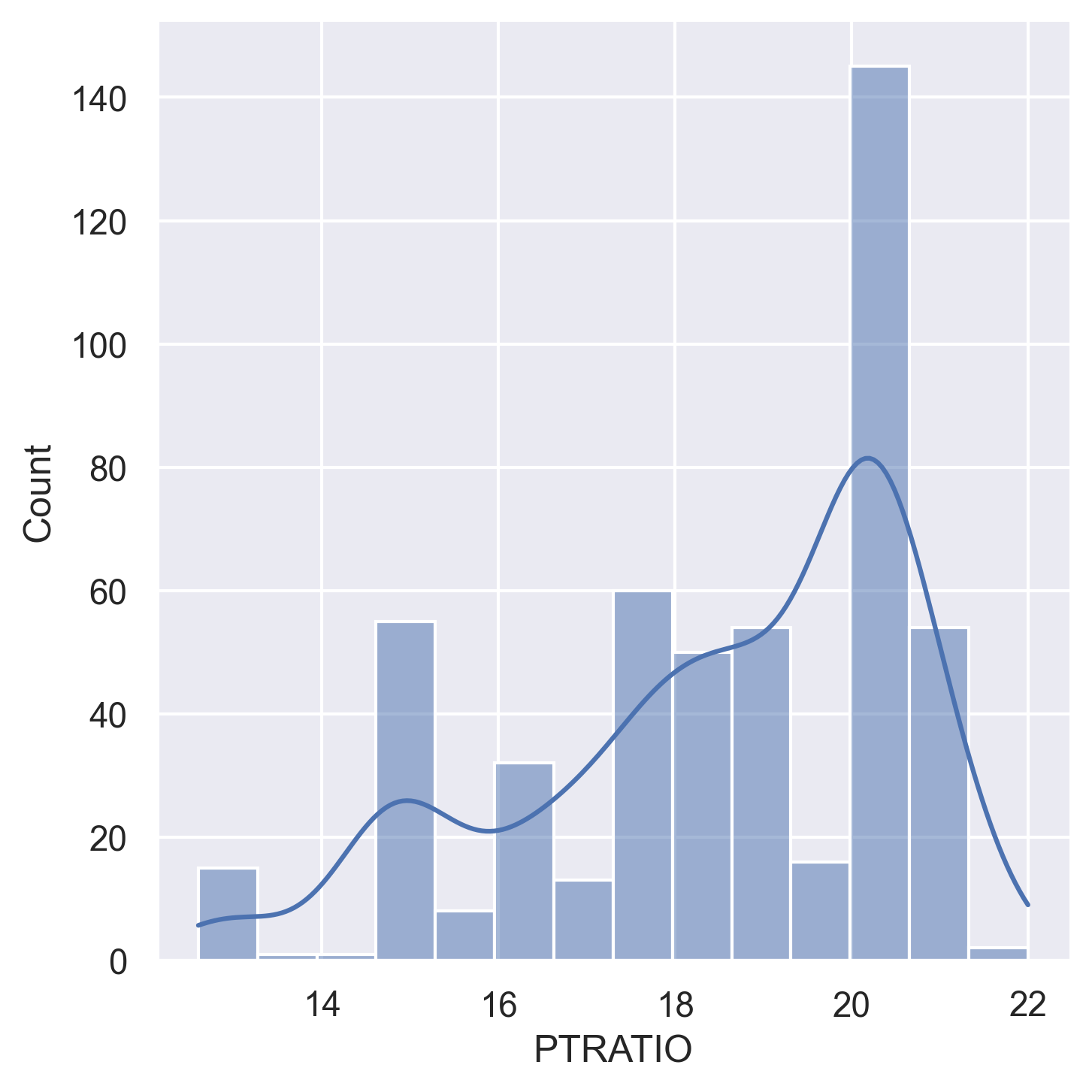 | 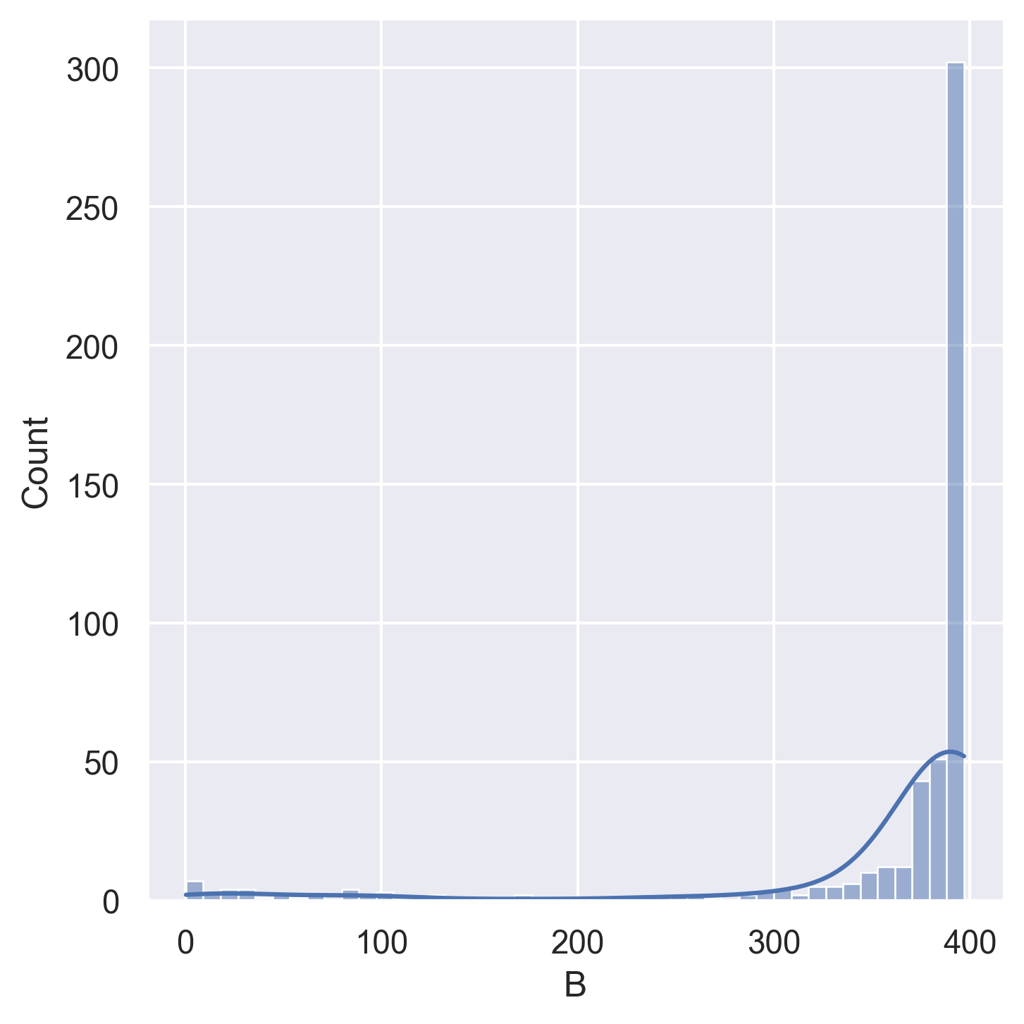 |
 |  |
Correlation Analysis
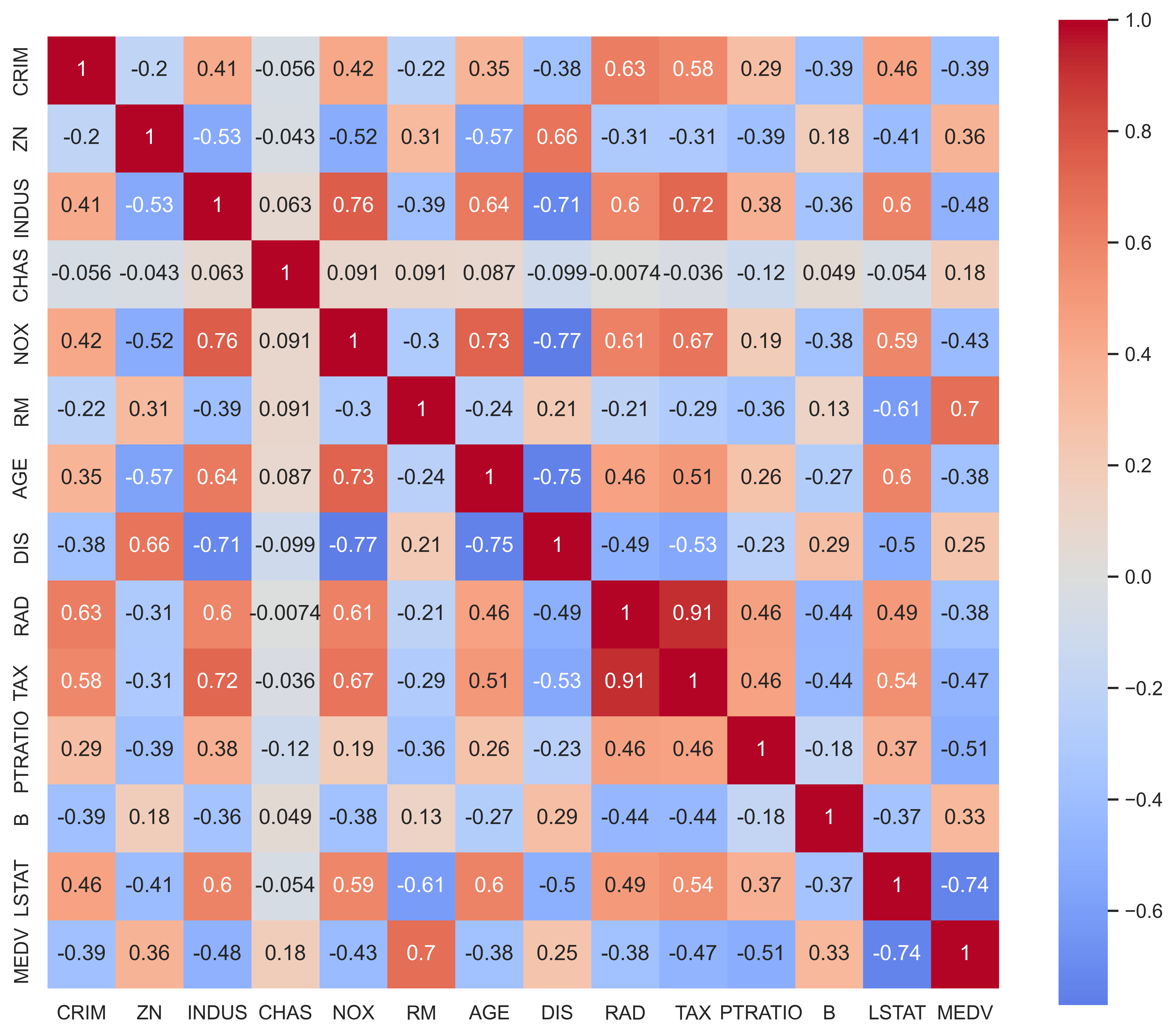 | 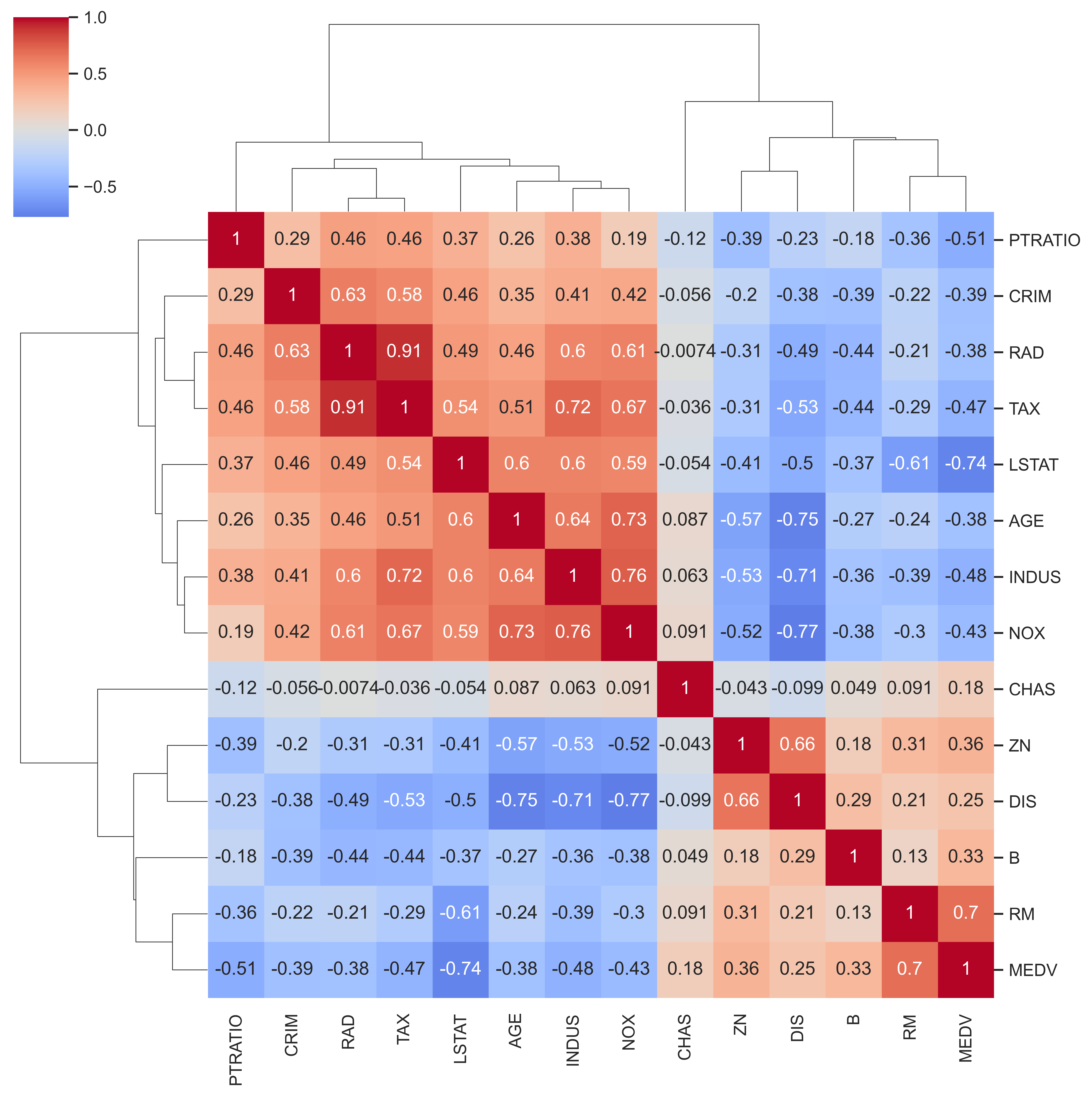 |
| Standard correlation heatmap | Hierarchical clustered correlation map |
Key correlations with MEDV (target):
- Strong positive:
RM(rooms) — more rooms → higher price - Strong negative:
LSTAT(lower status %) — higher LSTAT → lower price - Notable negatives:
PTRATIO,INDUS,TAX,CRIM
Methods Implemented
1. Gradient Descent — Linear Regression from Scratch (rawRun.py)
A pure NumPy implementation with no ML library abstractions:
- Manual weight initialisation (
w ~ N(0, 0.01),b = 0) - MSE loss with analytical gradient computation
- Convergence tolerance check (
tol = 1e-4) - Hyperparameters:
α = 0.001,epochs = 1200
# Core update rule (no libraries)
dw = (2 / m) * X_train.T @ (y_pred - y_train)
db = (2 / m) * sum(y_pred - y_train)
w -= α * dw
b -= α * db
2. Neural Network — Keras/TensorFlow (EvolutionaryAlgorithm.py)
A 3-hidden-layer dense network trained with Adam optimiser:
| Layer | Units | Activation |
|---|---|---|
| Input | 13 | — |
| Hidden 1 | 22 | ReLU |
| Hidden 2 | 22 | ReLU |
| Hidden 3 | 22 | ReLU |
| Output | 1 | Linear |
- Total parameters: 1,343
- Optimiser: Adam
- Loss: MSE
- Batch size: 32, Epochs: 50 (with early stopping, patience=20)
3. Evolutionary Algorithm (Work in Progress)
Scaffolded in EvolutionaryAlgorithm.py — evolves neural network weights using:
- Tournament selection (k=3)
- Gaussian mutation (per-gene with configurable rate and sigma)
- Uniform crossover (per-gene swap with configurable rate)
⚠️ Status: Skeleton implemented —
fitness(),ea_training_loop(), andmutation()functions are stubbed and awaiting completion.
Results Comparison
Metrics
| Metric | Gradient Descent (Linear) | Neural Network (Keras) | Evolutionary Algorithm |
|---|---|---|---|
| MSE | 32.406 | 12.957 | 101.712 |
| RMSE | 5.692 | 3.599 | 10.085 |
| MAE | 3.378 | 2.399 | 7.748 |
| R² | 0.558 | 0.823 | −0.387 |
Training Loss Curves
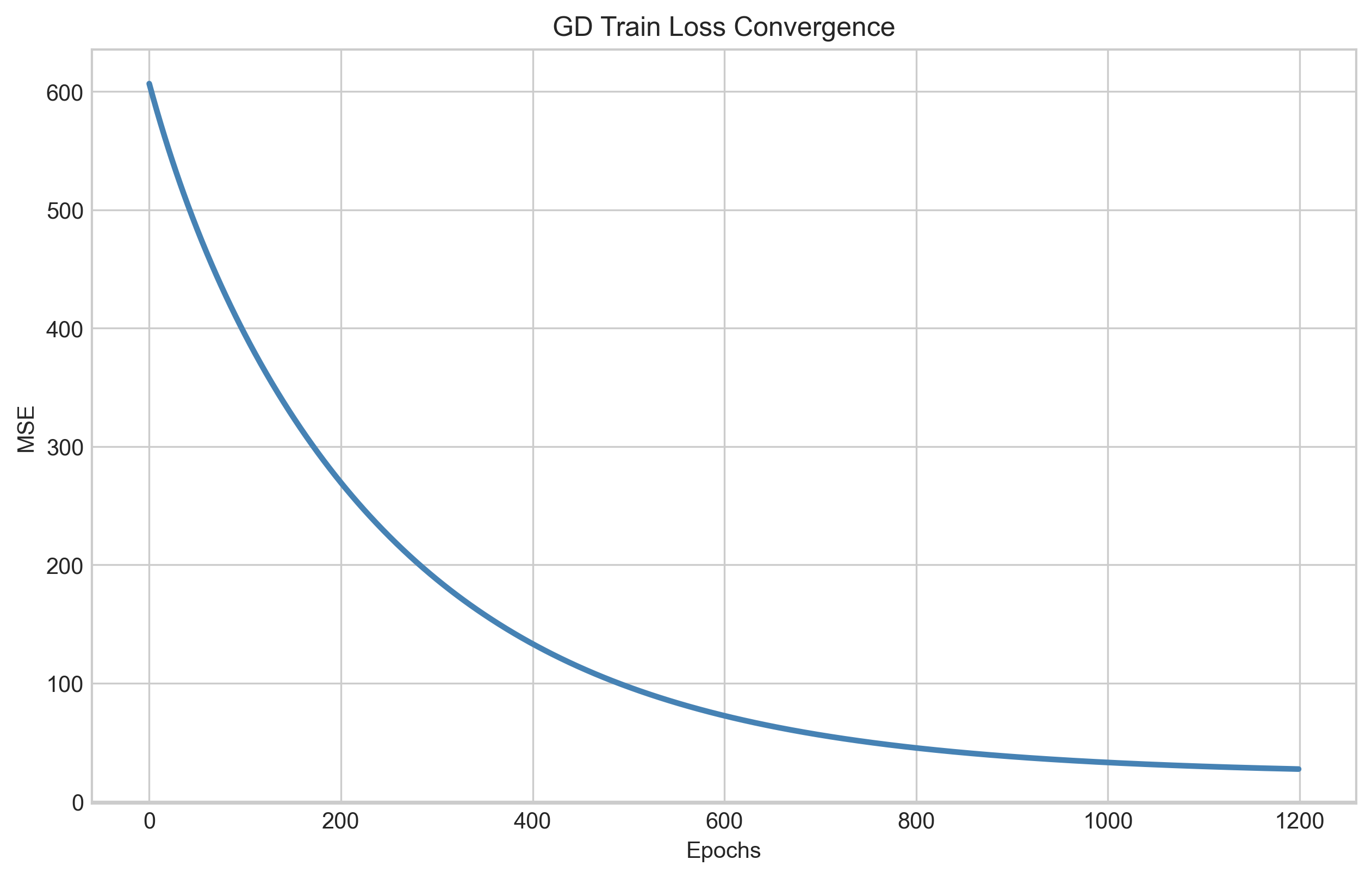 | 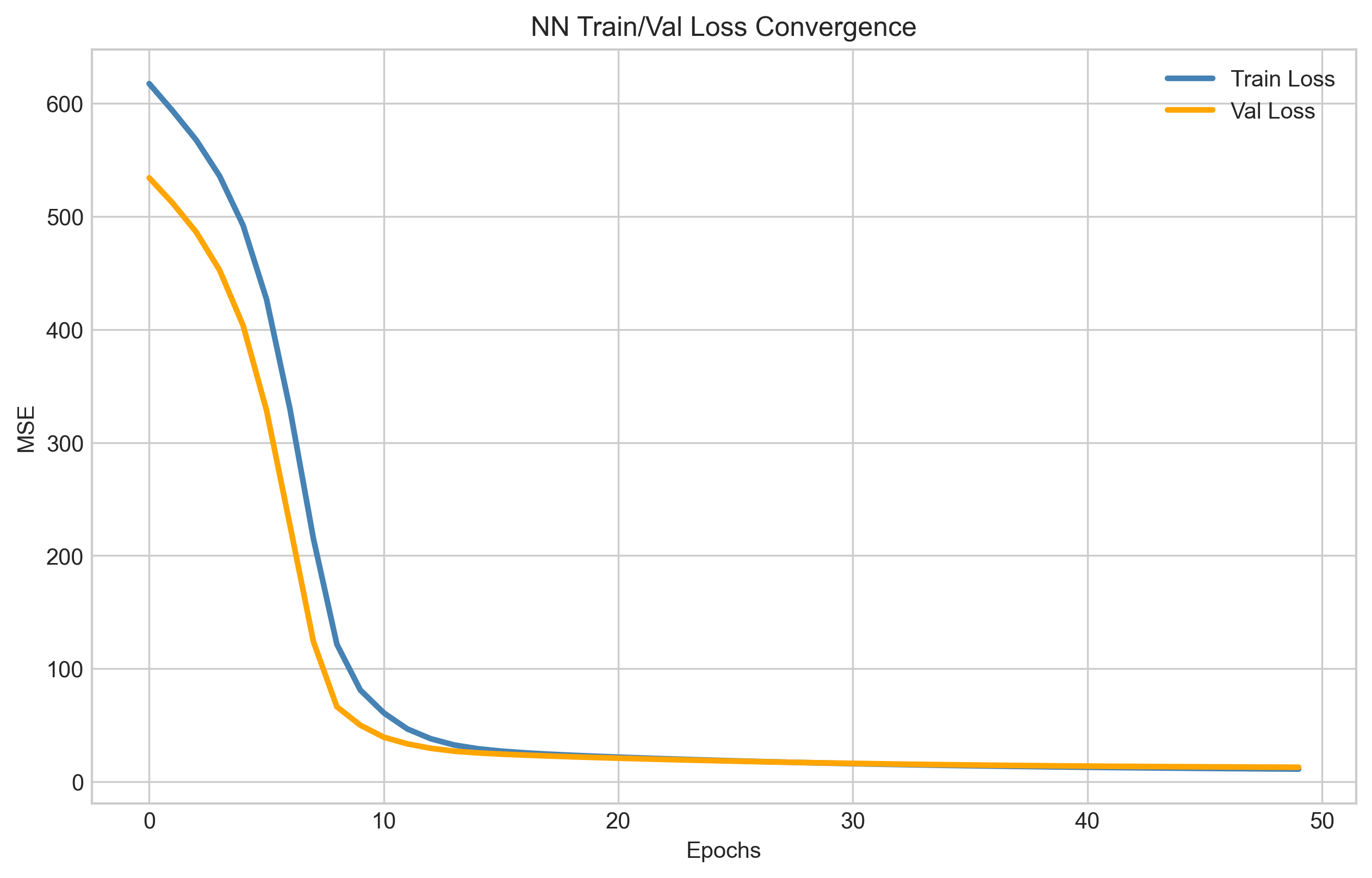 | 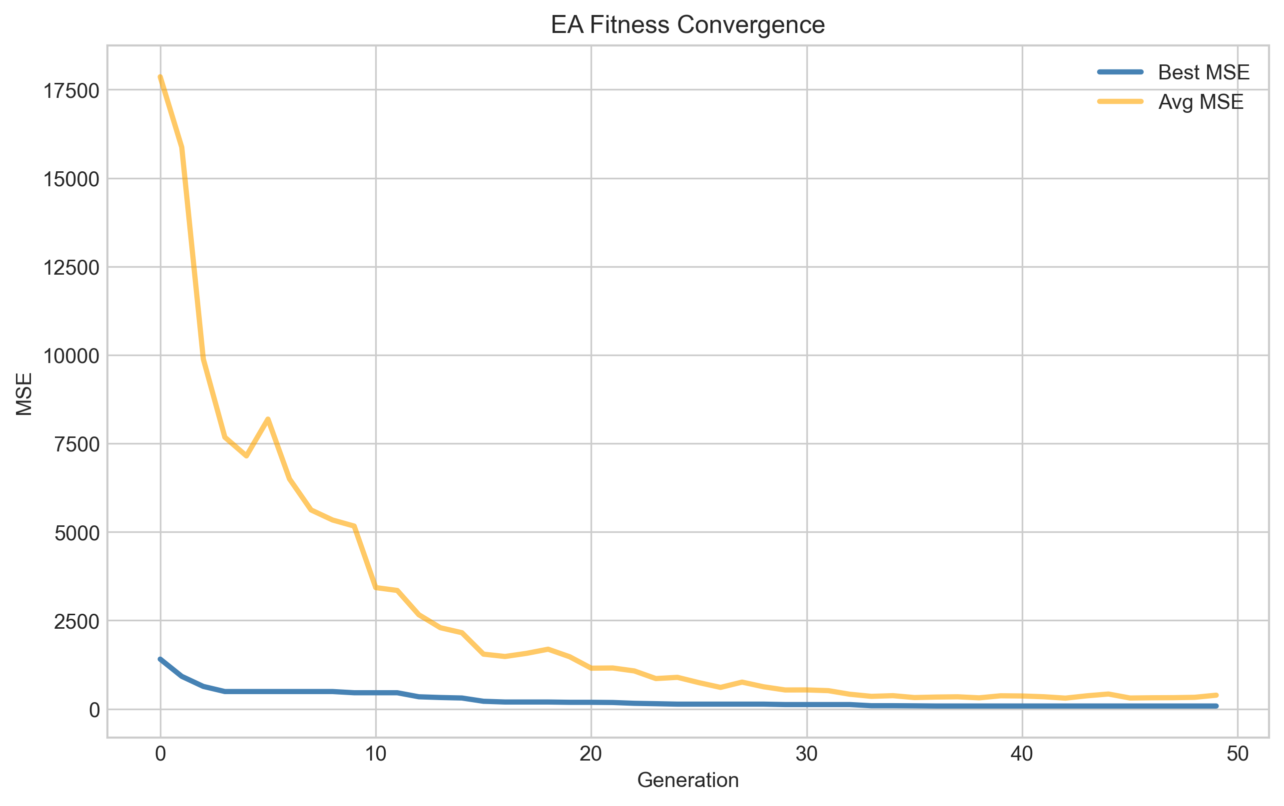 |
| Gradient descent MSE convergence over ~1200 epochs | NN train/validation loss over ~50 epochs (with early stopping) | EA fitness convergence over 50 generations |
Test Set Predictions — Actual vs Predicted
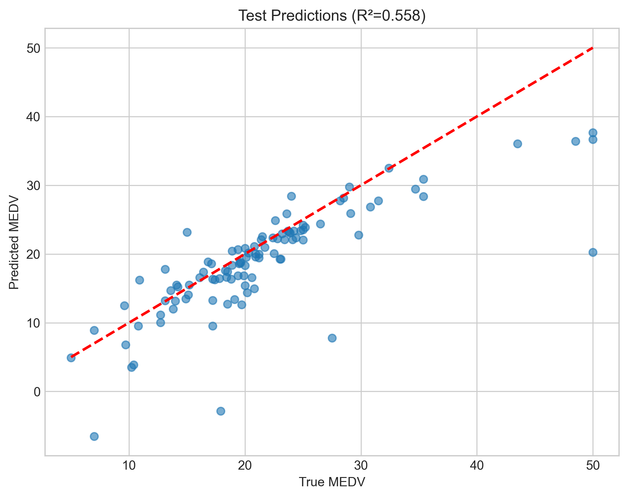 | 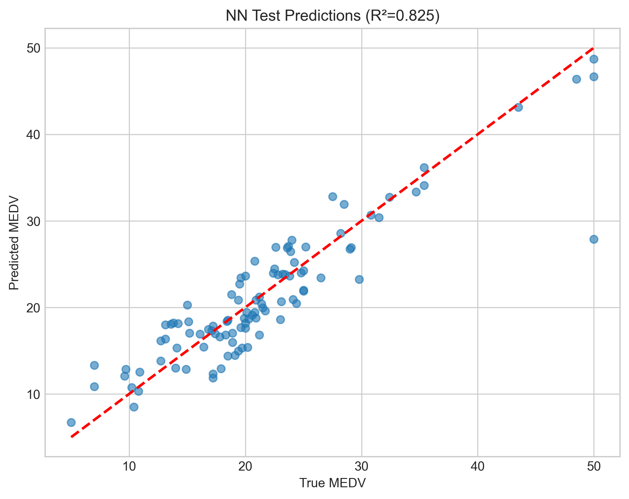 | 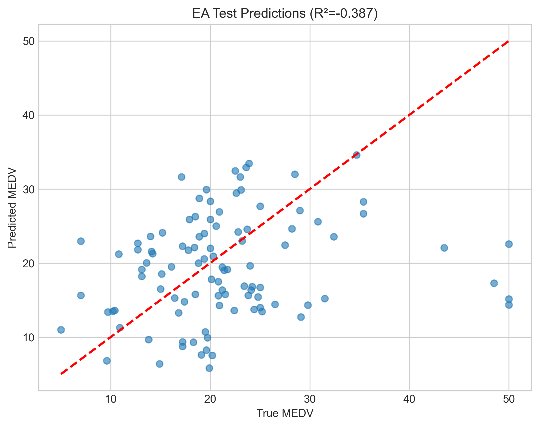 |
| Gradient descent predictions | Neural network predictions | Evolutionary algorithm predictions |
Points closer to the red dashed line (y = x) indicate better predictions. The neural network shows tighter clustering around the ideal line, especially in the mid-range values.
Project Structure
Zamin/
├── rawRun.py                 # Gradient descent linear regression (from scratch)
├── NeuralNetwork.py          # Neural network with Keras/TensorFlow
├── EvolutionaryAlgorithm.py  # Evolutionary algorithm for NN weight optimisation
├── dataPreProcess.py         # Dataset visualisation & correlation analysis
├── housing.csv               # Boston Housing dataset (506 × 14)
├── stickyNote.txt            # Project notes & core concepts
└── output/
    ├── dataanalysis/         # Histograms, heatmaps, correlation plots
    ├── linearreg/            # GD loss curves & scatter plots
    ├── nn/                   # NN loss curves, scatter plots & saved models
    └── ea/                   # EA convergence & prediction plots
Key Takeaways
The evolutionary algorithm failed spectacularly, I was rather surprised. I was expecting it to fall a bit short, but not underperform to this extent. Linear regression and te NN were a delight however, solid scores with very simple setups. I found the NN topology taken from the study to be straight forward to implement and logical.
Future Work
Lots of things could be improved, first and foremost add ridge regression to the linear algorithm, for the NN - add pruning. These are nice but most of all I will be looking to implement these onto a more sophisticated and real-world dataset. This project was great for the rapid feedback loop and small scale. Ramping up to something more fully fledged is the next step. Definitely more to come.